Page 63 - Numerical methods for chemical engineering

Sparse and banded matrices 49

In general, this approximation is not exact, and we must reduce the value of y by increasing
N until the magnitude of the approximation error is below some acceptable value. For this
particularproblem,asthetruesolutionisaquadraticfunction,weareluckyandthisalgebraic
approximation is exact.
To “solve” a boundary value problem using the method of finite differences, we formulate
a set of N algebraic equations for the set of N unknowns {v x (y 1 ),v x (y 2 ),...,v x (y N )}.For
each grid point, we obtain an algebraic equation by requiring the differential equation to be
satisfied locally

2
P d v x
0 =− + µ (1.245)
x dy 2
y j
If we insert the central-difference approximation for the second derivative, the algebraic
equation for grid point j is

P v x (y j+1 ) − 2v x (y j ) + v x (y j−1 )
0 =− + µ (1.246)
x ( y) 2
We write this in a more compact form by defining the column vector
   
v 1 v x (y 1 )
v x (y 2 )
v 2
   
    (1.247)
. 
v =  .  = 
.
 .   . . 
v N v x (y N )
so that the algebraic equation for grid point j becomes
( y) 2 P
v j+1 − 2v j + v j−1 = (1.248)
µ x
It is standard practice to make the diagonal elements positive,
( y) 2 P
−v j+1 + 2v j − v j−1 =− (1.249)
µ x
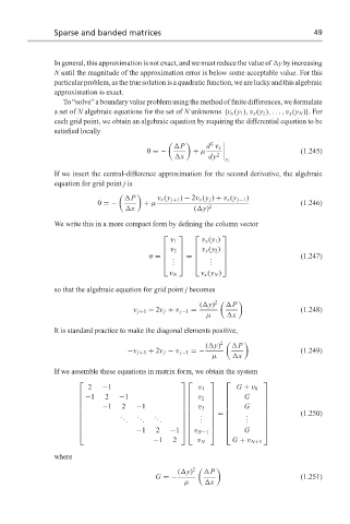
If we assemble these equations in matrix form, we obtain the system

     
2 −1 v 1 G + v 0
 −1 2 −1     G 



  v 2 
−1 2 −1 G
     
   v 3   
. . .
   .  =  .  (1.250)
 . . . . . .   . .   . . 
     
     
−1 2 G
 −1   v N−1   
−1 2 v N G + v N+1
where
( y) 2 P
G =− (1.251)
µ x