Page 61 - Numerical methods for chemical engineering

Sparse and banded matrices 47

B
v e
B
e e

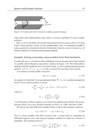
Figure 1.10 Pressure-driven flow between two infinite, parallel, flat plates.

makes them ideal building blocks upon which to construct algorithms for more complex
problems.
Here,wesolveaboundaryvalueproblemfromfluidmechanicsnumericallybyconverting
it into a linear algebraic system. As this example makes clear, it is sometimes possible to
reduce greatly the computational burden of elimination when the matrix is banded; i.e., all
nonzero elements are found near the principal diagonal.

Example. Solving a boundary value problem from fluid mechanics
Consider the case of a Newtonian fluid undergoing laminar, pressure-driven flow between
two parallel, infinite flat plates separated by a distance B (Figure 1.10). The bottom plate is
stationaryandthetopplatemovesataconstantvelocity V up .Foraconstantdynamicpressure
gradient, P/ x, P = p − g · r, we wish to calculate the resulting velocity profile.
If we assume a velocity profile of the form

v(r, t) = v x (y)e x (1.235)
the equation of continuity for an incompressible fluid, ∇ · v = 0, is satisfied automatically
and the Navier–Stokes equation of motion
Dv ∂
2
ρ = ρ v + ρv ·∇ v =−∇ P + µ∇ v (1.236)
Dt ∂t
reduces to
2
P d v x
0 =− + µ (1.237)
x dy 2
A brief discussion of these equations is provided in the supplemental material in the accom-
panying website. For a more detailed treatment, see Bird et al. (2002) and Deen (1998).
We wish to solve this differential equation subject to the no-slip boundary conditions

v x (y = 0) = 0 v x (y = B) = V up (1.238)

This is a classic problem from fluid mechanics that is solved easily by integrating the
differential equation twice and using the boundary conditions to obtain the constants of
integration. The resulting solution is
y 1 P 2
$ %
v x (y) = V up + (y − yB) (1.239)
B 2µ x