Page 69 - Numerical methods for chemical engineering

Sparse and banded matrices 55

A
1 1
1 1
2 2
1 2 1 2
n 1 n 22

1 1
1 1
2 2
1 2 1 2
n 22 n 22
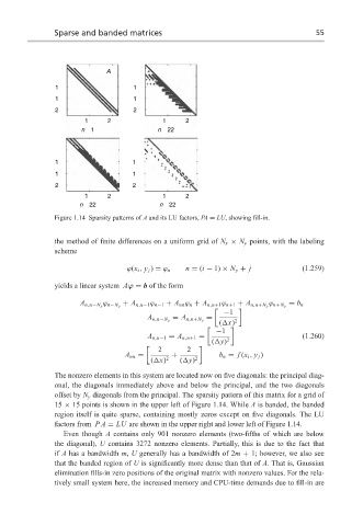
Figure 1.14 Sparsity patterns of A and its LU factors, PA = LU, showing fill-in.

the method of finite differences on a uniform grid of N x × N y points, with the labeling
scheme

ϕ(x i , y j ) = ϕ n n = (i − 1) × N y + j (1.259)

yields a linear system Aϕ = b of the form

ϕ ϕ
A n,n−N y n−N y + A n,n−1 ϕ n−1 + A nn ϕ n + A n,n+1 ϕ n+1 + A n,n+N y n+N y = b n

−1
=
A n,n−N y = A n,n+N y 2
( x)
−1

A n,n−1 = A n,n+1 = (1.260)
( y) 2

2 2
A nn = + b n = f (x i , y j )
( x) 2 ( y) 2
The nonzero elements in this system are located now on five diagonals: the principal diag-
onal, the diagonals immediately above and below the principal, and the two diagonals
offset by N y diagonals from the principal. The sparsity pattern of this matrix for a grid of
15 × 15 points is shown in the upper left of Figure 1.14. While A is banded, the banded
region itself is quite sparse, containing mostly zeros except on five diagonals. The LU
factors from PA = LU are shown in the upper right and lower left of Figure 1.14.
Even though A contains only 901 nonzero elements (two-fifths of which are below
the diagonal), U contains 3272 nonzero elements. Partially, this is due to the fact that
if A has a bandwidth m, U generally has a bandwidth of 2m + 1; however, we also see
that the banded region of U is significantly more dense than that of A. That is, Gaussian
elimination fills-in zero positions of the original matrix with nonzero values. For the rela-
tively small system here, the increased memory and CPU-time demands due to fill-in are