Page 35 - Optofluidics Fundamentals, Devices, and Applications

16 Cha pte r T w o

Dye 1
Dye 2
Microchannel wall

Dye 3
To outlet
Dye 4

200 μm
Dye 5
Dye 6
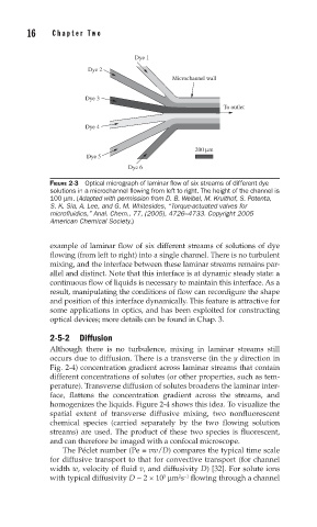
FIGURE 2-3 Optical micrograph of laminar fl ow of six streams of different dye
solutions in a microchannel fl owing from left to right. The height of the channel is
100 μm. (Adapted with permission from D. B. Weibel, M. Kruithof, S. Potenta,
S. K. Sia, A. Lee, and G. M. Whitesides, “Torque-actuated valves for
microfluidics,” Anal. Chem., 77, (2005), 4726–4733. Copyright 2005
American Chemical Society.)

example of laminar flow of six different streams of solutions of dye
flowing (from left to right) into a single channel. There is no turbulent
mixing, and the interface between these laminar streams remains par-
allel and distinct. Note that this interface is at dynamic steady state: a
continuous flow of liquids is necessary to maintain this interface. As a
result, manipulating the conditions of flow can reconfigure the shape
and position of this interface dynamically. This feature is attractive for
some applications in optics, and has been exploited for constructing
optical devices; more details can be found in Chap. 3.

2-5-2 Diffusion
Although there is no turbulence, mixing in laminar streams still
occurs due to diffusion. There is a transverse (in the y direction in
Fig. 2-4) concentration gradient across laminar streams that contain
different concentrations of solutes (or other properties, such as tem-
perature). Transverse diffusion of solutes broadens the laminar inter-
face, flattens the concentration gradient across the streams, and
homogenizes the liquids. Figure 2-4 shows this idea. To visualize the
spatial extent of transverse diffusive mixing, two nonfluorescent
chemical species (carried separately by the two flowing solution
streams) are used. The product of these two species is fluorescent,
and can therefore be imaged with a confocal microscope.
The Péclet number (Pe ≡ vw/D) compares the typical time scale
for diffusive transport to that for convective transport (for channel
width w, velocity of fluid v, and diffusivity D) [32]. For solute ions
with typical diffusivity D ~ 2 × 10 μm s flowing through a channel
3
2 −1