Page 180 - Orlicky's Material Requirements Planning

CHAPTER 8 Lot Sizing 159

EVALUATING LOT-SIZING TECHNIQUES

Every one of the lot-sizing techniques reviewed earlier is imperfect—each suffers from
some deficiency, as has been illustrated. In evaluating the relative effectiveness of these
techniques, the difficulty lies in the fact that the performance of the algorithms varies
depending on the net requirements data used and on the ratio of setup and unit costs.
Furthermore, some of the techniques assume gradual, steady-rate inventory depletion,
whereas others assume discrete depletion, which affects the way inventory carrying cost
would have to be computed for purposes of comparison. Ignoring this distinction and
basing all inventory carrying costs on discrete depletion at the beginning of each period,
the performance of the economics-oriented lot-sizing algorithms for which the same data
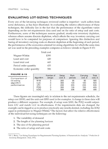
set was used in the preceding examples compares as follows (details in Figure 8-15):

Total cost
Wagner-Whitin $395
Least unit cost 420
Least total cost 445
Period order quantity 455
Economic order quantity 506

FIGURE 8-15
Number of Setup Part- Carrying Total
Comparison of Algorithm setups cost, $ periods cost, $ cost, $
lot-sizing W-W 3 300 95 95 395
algorithm LUC 3 300 120 120 420
performance. LTC 2 200 245 245 445
POQ 3 300 155 155 455
EOQ 3 300 206 206 506

These figures are meaningful only in relation to the net requirements schedule, the
setup cost ($100), and the unit cost ($50) used in the examples. A change in these data will
produce a different sequence. For example, if setup were $300, the POQ would outper-
form LTC and match LUC in effectiveness. If the requirements data are changed, the
example can be rigged so as to produce practically any results desired, including the EOQ
6
equal in performance to Wagner-Whitin. The factors that affect the relative effectiveness
of the individual lot-sizing techniques are the following:
1. The variability of demand
2. The length of the planning horizon
3. The size of the planning period
4. The ratio of setup and unit costs

6 W. L. Berry, “Lot Sizing Procedures for Requirements Planning Systems. A Framework for Analysis.” Production &
Inventory Management. 13(2), 1972.