Page 390 - Orlicky's Material Requirements Planning

CHAPTER 21 Historical Context 369

if different policies apply to a limited number of inventory groups. Under the conven-
tional approach to aggregate inventory management, the two inventory categories most
susceptible to control by means of varying a policy are lot-size inventory and safety stock.
When lot sizes are being determined through some form of the EOQ formula, it is possi-
ble to exert across-the-board control over them by manipulating the carrying-cost vari-
able in this formula.
Carrying cost, a controversial value, is in all cases semiarbitrary (in practice, the val-
ues in use vary between 8 and 45 percent per annum from company to company) and
therefore can be thought of as reflecting management policy. Increasing the carrying cost
used in the EOQ computation will result in smaller lot sizes, and vice versa. Thus the
inventory carrying cost in use at any given time reflects the premium that management
is putting on the conservation of cash.
The idea is entirely sound, and its application is simple and direct. This brings the
focus to the real driving force behind establishment of lot size, which is the setup time.
The other factors in the EOQ equation (i.e., carrying cost, annual usage, and inventory
carrying cost) are out of the direct control of the operations manager. The only item that
can be affected directly by operations is the setup time to result in a reduced EOQ lot size.
This is the basis for the single minute exchange of dies (SMED) that is so essential in lean
implementations.
What now must be discarded, however, are the traditional methods of quantifying
the results that can be expected as a consequence of a given individual policy change. In
an EOQ environment, the theoretical relationship between incremental change in carry-
ing cost and lot-quantity change (and, by extension, lot-size inventory change) is clean
and straightforward. The EOQ varies inversely with the square root of the carrying cost.
The value of EOQ squared doubles as a result of halving carrying costs and halves as a
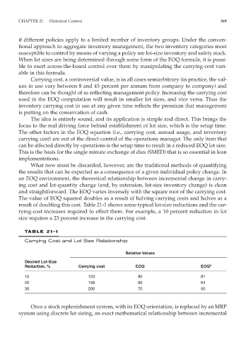
result of doubling this cost. Table 21-1 shows some typical lot-size reductions and the car-
rying-cost increases required to effect them. For example, a 10 percent reduction in lot
size requires a 23 percent increase in the carrying cost.

TA B LE 21-1
Carrying Cost and Lot Size Relationship

Relative Values
Desired Lot-Size
Reduction, % Carrying cost EOQ EOQ 2

10 123 90 81
20 156 80 64
30 200 70 50

Once a stock replenishment system, with its EOQ orientation, is replaced by an MRP
system using discrete lot sizing, an exact mathematical relationship between incremental