Page 111 -

98 4 Statistical Classification

respectively. Figure 4.18 illustrates the normal distribution for the two-dimensional
situation.
Given a training set with n patterns T=(x,, x2, .., x,} characterized by a
distribution with pdfp(q8 ), where 8 is a parameter vector of the distribution (e.g.
the mean vector of a normal distribution), an interesting way of obtaining sample
estimates of the parameter vector 8 is to maximize p(q8 ), which viewed as a
function of 8 is called the likelihood of 8 for the given training set. Assuming that
each pattern is drawn independently from a potentially infinite population, we can
express this likelihood as:

When using the maximum likelihood estimation of distribution parameters it is
often easier to compute the maximum of ln[p(qB )], which is equivalent (the
logarithm is a monotonic increasing function). For Gaussian distributions, the
sample estimates given by formulas (4-21a) and (4-21b) are maximum likelihood
estimates and will converge to the true values with an increasing number of cases.
The reader can find a detailed explanation of the parameter estimation issue in
Duda and Hart (1973).
As can be seen from (4-21), the surfaces of equal probability density for normal
likelihood satisfy the Mahalanobis metric already discussed in sections 2.2, 2.3 and
4.1.3.

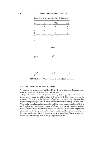
Figure 4.18. The bell-shaped surface of a two-dimensional normal distribution.
An ellipsis with equal probability density points is also shown.

Let us now proceed to compute the decision function (4-l8d) for normally
distributed features:

We may apply a monotonic logarithmic transformation (see 2.1. I), obtaining: