Page 26 - Phase Space Optics Fundamentals and Applications

Wigner Distribution in Optics 7

Γ(r + r , r − r )
1
1
2 2

W(r,q) A(r,q )

Γ(q + q , q − q )
−
1
1
2 2
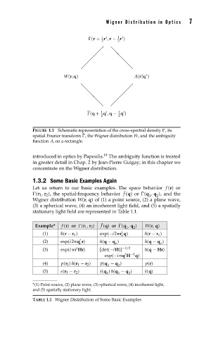
FIGURE 1.1 Schematic representation of the cross-spectral density , its
spatial Fourier transform ¯ , the Wigner distribution W, and the ambiguity
function A, on a rectangle.

introduced in optics by Papoulis. 19 The ambiguity function is treated
in greater detail in Chap. 2 by Jean-Pierre Guigay; in this chapter we
concentrate on the Wigner distribution.

1.3.2 Some Basic Examples Again
Let us return to our basic examples. The space behavior f (r)or
¯
(r 1 , r 2 ), the spatial-frequency behavior f (q)or ¯ (q , q ), and the
1 2
Wigner distribution W(r, q) of (1) a point source, (2) a plane wave,
(3) a spherical wave, (4) an incoherent light field, and (5) a spatially
stationary light field are represented in Table 1.1.

¯
Example* f (r) or (r 1 , r 2 ) f (q) or ¯ (q , q ) W(r, q)
1 2
t
(1) (r − r o ) exp(−i2 r q) (r − r o )
o
t
(2) exp(i2 q r) (q − q ) (q − q )
o o o
t
(3) exp(i r Hr) [det(−iH)] −1/2 (q − Hr)
t
exp(−i q H −1 q)
(4) p(r 1 ) (r 1 − r 2 ) ¯ p(q − q ) p(r)
1
2
(5) s(r 1 − r 2 ) ¯ s(q ) (q − q ) ¯ s(q)
1 1 2
∗ (1) Point source, (2) plane wave, (3) spherical wave, (4) incoherent light,
and (5) spatially stationary light.
TABLE 1.1 Wigner Distribution of Some Basic Examples