Page 30 - Phase Space Optics Fundamentals and Applications

Wigner Distribution in Optics 11

• the (partially coherent) rotationally symmetric case (H = hI,
G 1 = g 1 I, G 2 = g 2 I, G 0 = (g 2 − g 1 )I, with I the 2 × 2 identity
matrix)

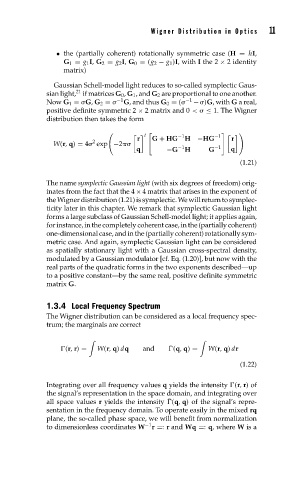
Gaussian Schell-model light reduces to so-called symplectic Gaus-
21
sian light, if matrices G 0 , G 1 , and G 2 are proportional to one another.
−1
Now G 1 =
G, G 2 =
G, and thus G 0 = (
−1 −
)G, with G a real,
positive definite symmetric 2 × 2 matrix and 0 <
≤ 1. The Wigner
distribution then takes the form

t −1 −1
r G + HG H −HG r
2
W(r, q) = 4
exp −2
−1 −1
q −G H G q
(1.21)
The name symplectic Gaussian light (with six degrees of freedom) orig-
inates from the fact that the 4 × 4 matrix that arises in the exponent of
the Wigner distribution (1.21) is symplectic. We will return to symplec-
ticity later in this chapter. We remark that symplectic Gaussian light
forms a large subclass of Gaussian Schell-model light; it applies again,
for instance, in the completely coherent case, in the (partially coherent)
one-dimensional case, and in the (partially coherent) rotationally sym-
metric case. And again, symplectic Gaussian light can be considered
as spatially stationary light with a Gaussian cross-spectral density,
modulated by a Gaussian modulator [cf. Eq. (1.20)], but now with the
real parts of the quadratic forms in the two exponents described—up
to a positive constant—by the same real, positive definite symmetric
matrix G.

1.3.4 Local Frequency Spectrum
The Wigner distribution can be considered as a local frequency spec-
trum; the marginals are correct

(r, r) = W(r, q) dq and ¯ (q, q) = W(r, q) dr

(1.22)

Integrating over all frequency values q yields the intensity (r, r)of
the signal’s representation in the space domain, and integrating over
all space values r yields the intensity ¯ (q, q) of the signal’s repre-
sentation in the frequency domain. To operate easily in the mixed rq
plane, the so-called phase space, we will benefit from normalization
−1
to dimensionless coordinates W r =: r and Wq =: q, where W is a