Page 377 - Phase Space Optics Fundamentals and Applications

358 Chapter Eleven

according to the inversion algorithm they employ for reconstructing
the ensemble statistics from the measured experimental trace. Phase-
space techniques estimate either the Wigner function or the ambiguity
function. There are two classes of phase-space techniques, spectro-
graphic and tomographic. Methods from which the inversion returns
either the two-time or two-frequency correlation function may be clas-
sified as direct techniques: these are interferometric.

11.3.2 Pulse Characterization Apparatuses
as Linear Systems
Although currently most methods for pulse characterization are based
on nonlinear optical processes, it is informative to consider a general
framework for analyzing measurement methods based on a linear
filter analysis. This approach has two benefits. First, it proves that
nonlinearities are not necessary for determining the pulse field and
shows why they are often used. Second, it specifies the necessary and
sufficient conditions that must be fulfilled by any apparatus that is ca-
pable of determining the field. This leads to a convenient classification
scheme for most methods.
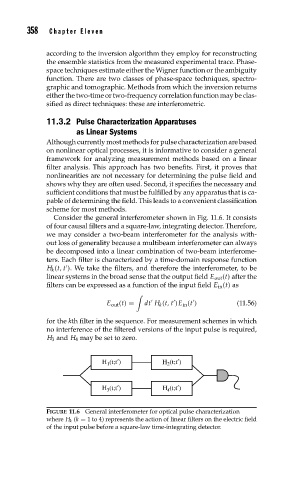
Consider the general interferometer shown in Fig. 11.6. It consists
of four causal filters and a square-law, integrating detector. Therefore,
we may consider a two-beam interferometer for the analysis with-
out loss of generality because a multibeam interferometer can always
be decomposed into a linear combination of two-beam interferome-
ters. Each filter is characterized by a time-domain response function
H k (t, t ). We take the filters, and therefore the interferometer, to be

linear systems in the broad sense that the output field E out (t) after the
filters can be expressed as a function of the input field E in (t)as

E out (t) = dt H k (t, t )E in (t ) (11.56)
for the kth filter in the sequence. For measurement schemes in which
no interference of the filtered versions of the input pulse is required,
H 3 and H 4 may be set to zero.

H (t;t′) H (t;t′)
2
1

H (t;t′) H (t;t′)
3
4
FIGURE 11.6 General interferometer for optical pulse characterization
where H k (k = 1 to 4) represents the action of linear filters on the electric field
of the input pulse before a square-law time-integrating detector.