Page 114 - Physical Principles of Sedimentary Basin Analysis

96 Burial histories

0

1000

depth [m] 2000

3000

(1) the used porosity
4000 (2) sand/sandstone (Baldwin & Butler, 1985)
(3) sand/sandstone (Helland−Hansen, 1988)
(4) shale (Baldwin & Butler, 1985)
(4) (5) (2) (3) (5) shale (Helland−Hansen, 1988)
(1)
5000
0 0.2 0.4 0.6 0.8
porosity [−]
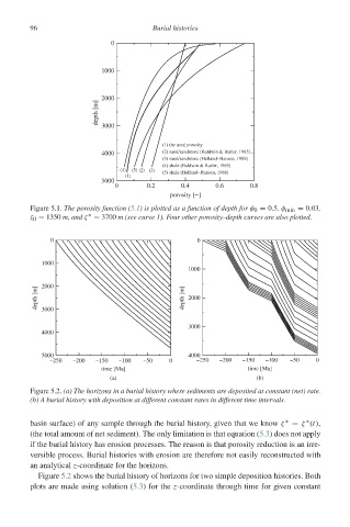
Figure 5.1. The porosity function (5.1) is plotted as a function of depth for φ 0 = 0.5, φ min = 0.03,
∗
ζ 0 = 1350 m, and ζ = 3700 m (see curve 1). Four other porosity–depth curves are also plotted.

0 0

1000
1000
depth [m] 2000 depth [m] 2000

3000
3000
4000

5000 4000
–250 –200 –150 –100 –50 0 −250 −200 −150 −100 −50 0
time [Ma] time [Ma]
(a) (b)
Figure 5.2. (a) The horizons in a burial history where sediments are deposited at constant (net) rate.
(b) A burial history with deposition at different constant rates in different time intervals.

∗
∗
basin surface) of any sample through the burial history, given that we know ζ = ζ (t),
(the total amount of net sediment). The only limitation is that equation (5.3) does not apply
if the burial history has erosion processes. The reason is that porosity reduction is an irre-
versible process. Burial histories with erosion are therefore not easily reconstructed with
an analytical z-coordinate for the horizons.
Figure 5.2 shows the burial history of horizons for two simple deposition histories. Both
plots are made using solution (5.3)forthe z-coordinate through time for given constant