Page 173 - Physical Principles of Sedimentary Basin Analysis

6.14 Instantaneous heating or cooling of semi-infinite half-space 155

instantaneous heating or cooling of the semi-infinite half-space is a useful starting point
for other similar problems, like cooling sills or dikes, and the thermal structure of the
lithosphere.
The semi-infinite half-space has a surface at z = 0 and it covers the entire z-axis below
the surface. The temperature of the half-space is initially at T 0 (for t < 0), but at t = 0the
surface temperature is suddenly changed to T s . The general temperature equation (6.15)
simplifies in this case to
2
∂T ∂ T
− κ = 0 (6.201)
∂t ∂z 2
where κ = λ/(c b b ) is the thermal diffusivity. The boundary conditions are the surface
temperature T (z=0, t) = T s and the temperature T = T 0 at infinite depth (for z →∞).
Note 6.7 shows that the solution of the temperature equation becomes

z
T (z, t) = T 0 + (T s − T 0 ) erfc √ , (6.202)
2 κt
where erfc(η) is a special function called the complementary error function. It is defined as

erfc(η) = 1 − erf(η) (6.203)
in terms of the error-function erf, which is given by the integral
√ η
π −x 2
erf(η) = e dx. (6.204)
2 0
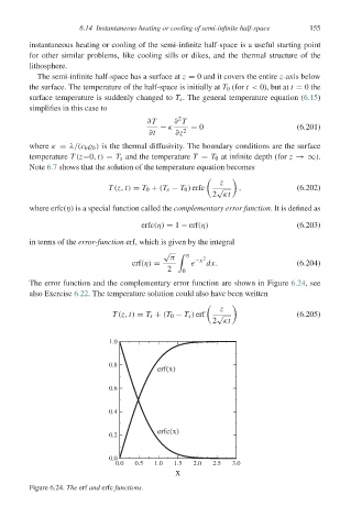
The error function and the complementary error function are shown in Figure 6.24,see
also Exercise 6.22. The temperature solution could also have been written
z

T (z, t) = T s + (T 0 − T s ) erf √ (6.205)
2 κt

1.0

0.8
erf(x)

0.6

0.4

erfc(x)
0.2

0.0
0.0 0.5 1.0 1.5 2.0 2.5 3.0
x
Figure 6.24. The erf and erfc functions.