Page 235 - Physical chemistry understanding our chemical world

202 PHASE EQUILIBRIA

so a graph of the form ‘y = mx + c’ is obtained by plotting ln p (as ‘y’) against
1/T (as ‘x’). The gradient of this Clapeyron graph is ‘− H O ÷ R’, so we obtain
(boil)
H O as ‘gradient ×−1 × R’.
(boil)
The intercept of a Clapeyron graph is not useful; its value may
We employ the inte- best be thought of as the pressure exerted by water boiling at infinite
grated form of the temperature. This alternative of the Clausius–Clapeyron equation
Clausius–Clapeyron is sometimes referred to as the linear (or graphical)form.
equation when we
know two tempera-
tures and pressures, Worked Example 5.3 The Clausius–Clapeyron equation need not
and the graphical form apply merely to boiling (liquid–gas) equilibria, it also describes sub-
for three or more. limation equilibria (gas–solid).
Consider the following thermodynamic data, which concern the sub-
limation of iodine:

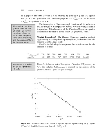
T (sublimation) /K 270 280 290 300 310 320 330 340
p (I 2 ) /Pa 50 133 334 787 1755 3722 7542 14 659

We obtain the value Figure 5.13 shows a plot of ln p (I 2 ) (as ‘y’) against 1/T (sublimation) (as
O
of H as ‘gradient× ‘x’). The enthalpy H is obtained via the gradient of the
(sublimation)
−1 × R’. graph 62 kJ mol −1 (note the positive sign).

−1

−2

−3

ln(p/Pa) −4

−5

−6

−7

−8
0.0029 0.0031 0.0033 0.0035 0.0037
K/T

Figure 5.13 The linear form of the Clausius–Clapeyron equation: a graph of ln p (as ‘y’) against
O
1/T (as ‘x’) should be linear with a slope of − H (vap) ÷ R