Page 303 - Physical Chemistry

lev38627_ch09.qxd 3/14/08 1:31 PM Page 284

284
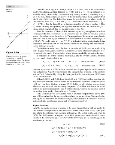
Chapter 9 The solid line in Fig. 9.20 shows m versus ln x at fixed T and P for a typical non-
i
i
Solutions electrolyte solution. At high dilutions (x
0.01 and ln x
4), the solution is es-
i i
sentially ideally dilute and m varies essentially linearly with ln x according to m
i i i
m° RT ln x . As ln x increases above 4, the solution deviates more and more from
i i i
ideally dilute behavior. The dashed line shows the hypothetical case where ideally di-
lute behavior holds as x → 1 and ln x → 0. The equation of the dashed line is m
i i i
m° RT ln x . For the dashed line, m becomes equal to m° when x reaches 1. Thus
i i i i i
m° can be found by extrapolating the high-dilution behavior of the solution to x 1.
i i
For an actual example of this, see the discussion of Fig. 9.21.
Since the properties of i in the dilute solution depend very strongly on the solvent
(which provides the environment for the i molecules), the fictitious standard state of
solute i depends on what the solvent is. The properties of the standard state also de-
pend on T and P, and m° is a function of T and P but not of the mole fractions: m°
i i
,A
m°(T, P). We might write m° m° (T, P) to indicate that the solute standard state
i i i
depends on the solvent, but we won’t do so unless we are dealing with solutions of i
in two different solvents.
The fictitious standard state of solute i is a state in which i is pure, but in which, by
some magical means, each i molecule experiences the same intermolecular forces it ex-
Figure 9.20 periences in the ideally dilute solution, where it is surrounded by solvent molecules.
In summary, the solute chemical potentials m and the solvent chemical potential
Chemical potential m plotted i
i
versus ln x for a typical m in an ideally dilute solution are
A
i
nonelectrolyte solute. The dashed
i
i
line extrapolates the ideally dilute m m°1T, P2 RT ln x for i A ideally dil. soln. (9.58)*
i
behavior to the limit x → 1. m m° RT ln x , m° m* 1T, P2 ideally dil. soln. (9.59)*
i
A
A
A
A
A
provided x is close to 1. The solvent standard state is pure liquid A at the tempera-
A
ture and pressure T and P of the solution. The standard state of solute i is the fictitious
state at T and P obtained by taking the limit x → 1 while pretending that (9.58) holds
i
for all concentrations.
Although (9.58) and (9.59) look like (9.42) and (9.43) for an ideal solution, ide-
ally dilute solutions and ideal solutions are not the same. Equations (9.58) and (9.59)
hold only for high dilution, whereas (9.42) holds for all solution compositions.
Moreover, the standard state for every component of an ideal solution is the actual
state of the pure component at T and P of the solution, whereas the standard state of
each solute in an ideally dilute solution is fictitious.
Some workers choose the standard state of solution components to have a pres-
sure of 1 bar, rather than the pressure of the solution as we have done. Since m of solids
and liquids is insensitive to pressure changes, this difference in choice of standard
states is of little significance unless high pressures are involved.
Vapor Pressure
Let P be the partial pressure of solute i in the vapor in equilibrium with an ideally di-
i
lute solution at temperature T and pressure P, where P equals the (total) vapor pres-
l
sure above the solution. The chemical potential m of i in the solution is given by
i
(9.58). We shall assume the vapor to be an ideal gas mixture, so the chemical poten-
v
v
tial of i in the vapor (v) is m m° (T) RT ln (P /P°) [Eq. (6.4)]. Equating m in the
i i i i
v
solution to m , we have
i
v
l
m m (9.60)
i
i
l
l
v
m° RT ln x m° RT ln 1P >P°2
i
i
i
i
l
l
v
1m° m° 2>RT ln 1P >x P°2
i
i
i
i
l
l
v
P >x P° exp31m° m° 2>RT4 (9.61)
i
i
i
i