Page 399 - Physical Chemistry

lev38627_ch12.qxd 3/18/08 2:41 PM Page 380

380
Chapter 12 Experimental Methods
Multicomponent Phase Equilibrium One way to determine a solid–liquid phase diagram experimentally is by thermal
analysis. Here, one allows a liquid solution (melt) of the two components to cool and
measures the system’s temperature as a function of time; this is repeated for several
liquid compositions to give a set of cooling curves. The time variable t is approxi-
mately proportional to the amount of heat q lost from the system, so the slope dT/dt
of a cooling curve is approximately proportional to the reciprocal of the system’s
heat capacity C dq /dT. Typical cooling curves for the simple eutectic system of
P P
Fig. 12.19 are shown in Fig. 12.27.
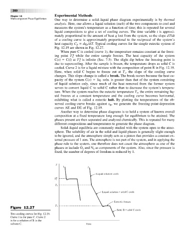
When pure C is cooled (curve 1), the temperature remains constant at the freez-
ing point T * while the entire sample freezes. The heat capacity of the system
C
C(s) C(l)at T * is infinite (Sec. 7.5). The slight dip below the freezing point is
C
due to supercooling. After the sample is frozen, the temperature drops as solid C is
cooled. Curve 2 is for a liquid mixture with the composition of point R in Fig. 12.19.
Here, when solid C begins to freeze out at T , the slope of the cooling curve
1
changes. This slope change is called a break. The break occurs because the heat ca-
pacity of the system C(s) liq. soln. is greater than that of the system consisting
of liquid solution only, since much of the heat removed from the former system
serves to convert liquid C to solid C rather than to decrease the system’s tempera-
ture. When the system reaches the eutectic temperature T , the entire remaining liq-
3
uid freezes at a constant temperature and the cooling curve becomes horizontal,
exhibiting what is called a eutectic halt. By plotting the temperatures of the ob-
served cooling-curve breaks against x ,we generate the freezing-point-depression
B
curves AE and DE of Fig. 12.19.
Another way to determine phase diagrams is to hold a system of known overall
composition at a fixed temperature long enough for equilibrium to be attained. The
phases present are then separated and analyzed chemically. This is repeated for many
different compositions and temperatures to generate the phase diagram.
Solid–liquid equilibria are commonly studied with the system open to the atmo-
sphere. The solubility of air in the solid and liquid phases is generally slight enough
to be ignored, and the atmosphere simply acts as a piston that provides a constant ex-
ternal pressure of 1 atm. The atmosphere is not part of the system, and in applying the
phase rule to the system, one therefore does not count the atmosphere as one of the
phases or include O and N as components of the system. Also, since the pressure is
2 2
fixed, the number of degrees of freedom is reduced by 1.

Figure 12.27
Two cooling curves for Fig. 12.19.
Curve 1 is for pure C. Curve 2
is for a solution of B in the
solvent C.