Page 76 - Physical Chemistry

lev38627_ch02.qxd 2/29/08 3:11 PM Page 57

57
Section 2.7
The Joule and
Joule–Thomson Experiments
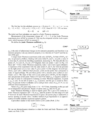
Figure 2.8

An isenthalpic curve obtained
from a series of Joule–Thomson
experiments.

The first law for this adiabatic process (q 0) gives U U q w w, so
2 1
U U P V P V or U P V U P V . Since H U PV, we have
1 1
1
2
2 2
1
1 1
2
2 2
H H or ¢H 0
2 1
The initial and final enthalpies are equal in a Joule–Thomson expansion.
Measurement of the temperature change T T T in the Joule–Thomson
2
1
experiment gives T/ P at constant H. This may be compared with the Joule experi-
ment, which measures T/ V at constant U.
We define the Joule–Thomson coefficient m by
JT
0T
m a b (2.64)*
JT
0P H
m is the ratio of infinitesimal changes in two intensive properties and therefore is an
JT
intensive property. Like any intensive property, it is a function of T and P (and the na-
ture of the gas).
A single Joule–Thomson experiment yields only ( T/ P) .Tofind( T/ P) val-
H
H
ues, we proceed as follows. Starting with some initial P and T ,we pick a value of
1
1
P less than P and do the throttling experiment, measuring T .We then plot the two
2
1
2
points (T , P ) and (T , P )ona T-P diagram; these are points 1 and 2 in Fig. 2.8.
1
1
2
2
Since H 0 for a Joule–Thomson expansion, states 1 and 2 have equal enthalpies.
A repetition of the experiment with the same initial P and T but with the pressure
1
1
on the right piston set at a new value P gives point 3 on the diagram. Several repe-
3
titions, each with a different final pressure, yield several points that correspond to
states of equal enthalpy. We join these points with a smooth curve (called an isen-
thalpic curve). The slope of this curve at any point gives ( T/ P) for the tempera-
H
ture and pressure at that point. Values of T and P for which m is negative (points to
JT
the right of point 4) correspond to warming on Joule–Thomson expansion. At point
4, m JT is zero. To the left of point 4, m JT is positive, and the gas is cooled by throt-
tling. To generate further isenthalpic curves and get more values of m (T, P), we use
JT
different initial temperatures T .
1
Values of m for gases range from 3 to 0.1°C/atm, depending on the gas and
JT
on its temperature and pressure. Figure 2.9 plots some m data for N gas.
2
JT
Joule–Thomson throttling is used to liquefy gases. For a gas to be cooled by a
Joule–Thomson expansion ( P 0), its m must be positive over the range of T and
JT
P involved. In Joule–Thomson liquefaction of gases, the porous plug is replaced by a
narrow opening (a needle valve). Another method of gas liquefaction is an approxi-
mately reversible adiabatic expansion against a piston.
A procedure similar to that used to derive (2.63) yields (Prob. 2.35a)
0H
a b C m JT (2.65) Figure 2.9
P
0P T
The Joule–Thomson coefficient
We can use thermodynamic identities to relate the Joule and Joule–Thomson coeffi- of N (g) plotted versus P and
2
cients; see Prob. 2.35b. versus T.