Page 66 - Plastics Engineering

Mechanical Behaviour of Plastics 49

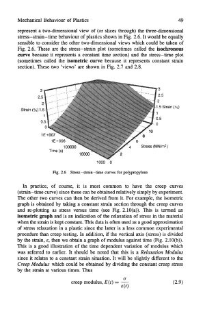
represent a two-dimensional view of (or slices through) the three-dimensional
stress-strain-time behaviour of plastics shown in Fig. 2.6. It would be equally
sensible to consider the other two-dimensional views which could be taken of
Fig. 2.6. These are the stress-strain plot (sometimes called the isochronous
curve because it represents a constant time section) and the stress-time plot
(sometimes called the isometric curve because it represents constant strain
section). These two 'views' are shown in Fig. 2.7 and 2.8.

Strain

1000 "'0
Fig. 2.6 Stress-strain-time curves for polypropylene

In practice, of course, it is most common to have the creep curves
(strain-time curve) since these can be obtained relatively simply by experiment.
The other two curves can then be derived from it. For example, the isometric
graph is obtained by taking a constant strain section through the creep curves
and re-plotting as stress versus time (see Fig. 2.10(a)). This is termed an
isometric graph and is an indication of the relaxation of stress in the material
when the strain is kept constant. This data is often used as a good approximation
of stress relaxation in a plastic since the latter is a less common experimental
procedure than creep testing. In addition, if the vertical axis (stress) is divided
by the strain, E, then we obtain a graph of modulus against time (Fig. 2.1O(b)).
This is a good illustration of the time dependent variation of modulus which
was referred to earlier. It should be noted that this is a Relaxation Modulus
since it relates to a constant strain situation. It will be slightly different to the
Creep Modulus which could be obtained by dividing the constant creep stress
by the strain at various times. Thus
fY
creep modulus, E(t) = - (2.9)
E@)