Page 36 - Power Electronic Control in Electrical Systems

//SYS21/F:/PEC/REVISES_10-11-01/075065126-CH001.3D ± 26 ± [1±30/30] 17.11.2001 9:43AM

26 Electrical power systems ± an overview

In addition to the large currents flowing from the generators to the point in fault fol-
lowing the occurrence of a three-phase short-circuit, the voltage drops to extremely
low values for the duration of the fault. The greatest voltage drop takes place at the
point in fault, i.e. zero, but neighbouring locations will also be affected to varying
degrees. In general, the reduction in root mean square (rms) voltage is determined by
the electrical distance to the short-circuit, the type of short-circuit and its duration.
The reduction in rms voltage is termed voltage sag or voltage dip. Incidents of this
are quite widespread in power networks and are caused by short-circuit faults, large
motors starting and fast circuit breaker reclosures. Voltage sags are responsible for
spurious tripping of variable speed motor drives, process control systems and com-
puters. It is reported that large production plants have been brought to a halt by sags
of 100 ms duration or less, leading to losses of hundreds of thousands of pounds
(McHattie, 1998). These kinds of problems provided the motivation for the devel-
opment of Custom Power equipment (Hingorani, 1995).

1.5.4 Random nature of system load

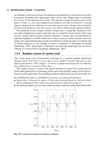
The system load varies continuously with time in a random fashion. Significant
changes occur from hour to hour, day to day, month to month and year to year
(Gross and Galiana, 1987). Figure 1.20 shows a typical load measured in a distribu-
tion substation for a period of four days.
The random nature of system load may be included in power flow studies and this
finds useful applications in planning studies and in the growing `energy stock market'.
Some possible approaches for modelling random loads within a power flow study are:

. modelling the load as a distribution function, e.g. normal distribution;
. future load is forecast by means of time series analysis based on historic values,
then normal power flow studies are performed for each forecast point;
. the same procedure as in two but load forecasting is achieved using Neural Networks.

0.50

0.40

[p.u.] 0.30

0.20

0.10

0.00
0 Sun 24 Mon 48 Tues 72 Wed 96

Hours
Fig. 1.20 A typical load measured at a distribution substation.