Page 345 - Pressure Swing Adsorption

r ,
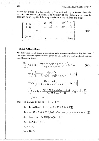
322 PRESSURE SWlNG ADSORPTION l APPENDIX B
I
l 323
collocauon points Z 2 , Z_~, ... , ZM+ . The exit velocity 1s known from the The collocation form of the particle balance equations 1s:
1
specified boundary condition. The velocity at the column inlet may be
8xCA ( . ]
obtained by soivrng the following matrix constructed from Eq. B.35: -- J' IC) = -,----c;---;--c---....,...,-;-;- ( B.39)
ar 1-xCA(J,k)-xc (J,k)
8
1 z, Z' zM g, "
c(2) 2 2
I z, Zi zr g,
i'(3)
+xCA(J,k) ,~, B(k,i)xc 8U,i))
(B.37) N+! '
"( M + 2) I
lM+I + .2
[1 -x,j1,k) -XcnC1,k)]

B.4.2 Other Steps
The followmg set Or linear aigebra1c equations 1s obtained when EQ. B.22 and
the velocity boundary condit10ns given by Eq. B.25 are combined and wntten
in collocat1on form:

~• [A ( .. ) _ Ax(M + 2,i)Ax(J,M + 2) ]-(·) _
+ ~t: A( k, i)Xcn(J, i))
,':'2 X J, l Ax( M + 2, M + 2) V l - (B.38)

axc"(1,k) = . -- '. YK .
a, t -,cAll,k) -xc (1,k) (B.40)
8
x([l -xcA(J,k)l~f B(k,i)xc/l(J,i)

+xca(1,k) ~t: B(k,i)xCA(J,i))
-(· (. I) _ Ax(J, M + 2)Ax(M + 2, 1) )-(l) _ .!_ ap
AXJ, Ax(M+2,M+2) / p·a,
+ YK
[1-xcA(J,k) -xc (1,k)]'
J = 2, ... , M + I 8
( N+ I
v(M + 2) is given by Eq. B.15. In Eq. B.33:
x([l-xcA(J,k)I ,~ A(k,i)xc 8 (1,i)
A,= 1/(Ax(J, M + 2) - (A Ax(M + 2, M + 2)]} N+ I \
3
+xc/l(J,k) ,~, A(k,i)xcA(J,i)j
A 2 = Ax(M+ 2,M + 2)/(Ax(l,M+2) - [A Ax(M +2,M + 2)]}
3
A 3 =[Ax(l,i)-Peii(l)]/Ax(M+2,l) X ( ~t: A(k, i)xc8(1, i)
A,= 1/Ax(M + 2, 1) l
N+ I
+ L A(k,i)xcA(1,i) ,
,. ' I
J = 2, ... , M + I; k = I, ... , N
Qm=W/Pe
xcjf, N + I) and xcsil, N + 1) arc obtained from Eos. B.42 and B.43.