Page 98 - Principles and Applications of NanoMEMS Physics

86 Chapter 3

ª E U 1( − e −ika 2 ) º
/
H = « s » , (11)
I « U 1 − e −ika 2/ ) E »
(
¬ p ¼
H Ψ = EΨ , (12)
I I I
B W B
B W B
B W B
Left Cladding B W B
Left Cladding
Right Cladding
Right Cladding
III
III
III II II II II I I I I
III
INCOMING
INCOMING
E E E c c c c
E z() z() z() z()
REFLECTED
REFLECTED
TRANSMITTED
TRANSMITTED ∆ ∆ E c z() z() z() z()
∆ E E
∆ E c c c
. . . GaAsGa AsAl . . . AlAsGaAs . . GaAsAlAs . . AlAsGaAsGaAs . . .. . . GaAsGa AsAl . . . AlAsGaAs . . GaAsAlAs . . AlAsGaAsGaAs . . . . . GaAsGa AsAl . . . AlAsGaAs . . GaAsAlAs . . AlAsGaAsGaAs . . . . . GaAsGa AsAl . . . AlAsGaAs . . GaAsAlAs . . AlAsGaAsGaAs . . .
. .
0 1 2 . . . n-1 n n+1 . . .
0 1 2 . . . n-1 n n+1 . . .
0 1 2 . . . n-1 n n+1 . . .
0 1 2 . . . n-1 n n+1 . . .
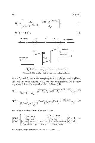
Figure 3-5. RTD structure for two-band tight-binding modeling.
where E and E are orbital energies prior to coupling to next neighbors,
P
S
and a is the lattice constant. Next, solutions are formulated for the three
regions as follows. For region I, we have (13) and (14).
Ψ L = 1 ( E − E φ + i E − E e − k i (a ) 4 / φ (13)
I 2E − E − E p s s ) p
s p
Ψ R = 1 ( E − E φ i − E − E e k i − (a ) 4 / φ (14)
I 2E − E − E p s s ) p
s p

For region II we have the transfer matrix (15).

E
1
ª U (n − ,n − ) E p (n − ) − (n ) º
1
1
ªC s (n º ) « » ªC s (n −1 º ) (15)
1
1
« » = « « U (n − ,n ) U (n − ,n ) » » « »
« ¬ C p (n ) » ¼ « [ − EE s (n ) ] (nU − ,1 n − )1 U (n − ,1 n ) + [ − EE s (n ][ ) E p (n − )1 − E ] « C p (n −1 » ) ¼
¬
»
1
« ¬ U (n ,n )U (n − ,n ) U (n , ) n U (n ,n )U (n − ,1 n ) » ¼
For coupling regions II and III we have (16) and (17).