Page 99 - Principles and Applications of NanoMEMS Physics

3. NANOMEMS PHYSICS: Quantum Wave Phenomena 87

Ψ = C φ + C φ = C Ψ L + C Ψ R (16)
III s s p p L III R III

ª 1 −i º
« −ika 2/ ika 4/ −ika 4/ »
ªC º « E −E 1( +e ) E −E ( e +e ) ª » C s º (17)
p
s
« L » = 2 E −E s −E p « « » »
« C » « 1 i « » C » p
¬ R ¼ ¬ ¼
« E −E 1( +e ika 2/ ) E −E ( e ika +e −ika 4/ ) »
« ¬ p s » ¼
The dispersion relation, velocity, and overlap integral defining the tight-
binding are given by (18), (19), and (20).

¨ ±
k ( E ) = § 4 · ¸ arcsin ª 1 ( E − E )( E − E p º » (18)
s
«
¨
¸
2
© a ¹ ¬ U ¼
v = ± aU 2 sin( ka ) 2 / (19)
= 2 ( E − E − E p )
s
2= 2 (E s − E p )
U = (20)
m * a 2
Finally, the current is given by (21), where x = E kT .

2 ∞ v k § ¨ 1 + e ( E F / kT − x) · ¸ (21)
e(
kT )
⋅
J ( V ) = ³ dx 2 ⋅ I ⋅ III ln ¨ ¸
4π 2 = 0 2 = v ¨ ¨ ª « E −eV /) kT − º » x ¸ ¸
(
C v III 1 « ¬ F » ¼
L III © + e ¹
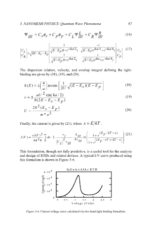
This formulation, though not fully predictive, is a useful tool for the analysis
and design of RTDs and related devices. A typical I-V curve produced using
this formalism is shown in Figure 3-6.
In Ga As/AlA s R T
In Ga As/AlA s R T D D
4 4
4 10
4 10 4 4
Current (A/cm2) Current (A/cm2) 3 10 4 4 4 4
3 10
2 10
2 10
1 10
1 10
0 0
0 0 0.5 1 1 1.5 2 2 2.5 3 3
1.5
2.5
0.5
V o lta g e (V o lts) )
V o lta g e (V o lts
Figure 3-6. Current-voltage curve calculated via two-band tight-binding formalism.