Page 238 - Principles of Applied Reservoir Simulation 2E

Part III: Case Study 223

to model the reservoir shown in Figure 21-2. Each gridblock is a square with
lengths A* = A>> = 200 ft. The dark areas of the grid are outside the reservoir
area. The pore volume in the dark area is made inactive in data file CS-HM.DAT
by using porosity multipliers.
The depth and thickness of each gridblock depend on reservoir architec-
ture. The model grid should approximate the structure depicted in Figure 21 -4,
which is based on Figures 20-1 and 20-2. The dip of the reservoir is included
by specifying the tops of each gridblock. The gridblock length modifications
are designed to cut off those parts of the block that continue the grid beyond the
surface of the unconformity sketched in Figure 21-4.
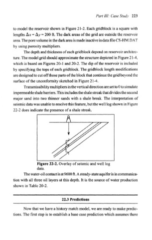
Transmissibility multipliers in the vertical direction are set to 0 to simulate
impermeable shale barriers. This includes the shale streak that divides the second
major sand into two thinner sands with a shale break. The interpretation of
seismic data was unable to resolve this feature, but the well log shown in Figure
22-2 does indicate the presence of a shale streak.

Figure 22-2. Overlay of seismic and well log
data.
The water-oil contact is at 9600 ft. A steady-state aquifer is in communica-
tion with all three oil layers at this depth. It is the source of water production
shown in Table 20-2.

22.3 Predictions

Now that we have a history match model, we are ready to make predic-
tions. The first step is to establish a base case prediction which assumes there