Page 322 - Principles of Applied Reservoir Simulation 2E

Part V: Technical Supplements 307

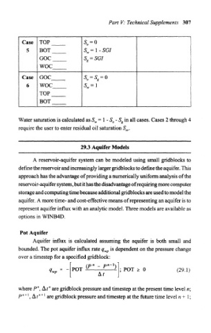
Case TOP S 0 = 0
5 EOT S w=l-SGI
GOC S g = SGI
woe

Case GOC S 0 = S g = Q
6 woe S w=l
TOP
BOT

Water saturation is calculated as S w = 1 - S 0 - S g in all cases. Cases 2 through 4
require the user to enter residual oil saturation S or.

29.3 Aquifer Models

A reservoir-aquifer system can be modeled using small gridblocks to
define the reservoir and increasingly larger gridblocks to define the aquifer. This
approach has the advantage of providing a numerically uniform analysis of the
reservoir-aquifer system, but it has the disadvantage of requiring more computer
storage and computing time because additional gridblocks are used to model the
aquifer. A more time- and cost-effective means of representing an aquifer is to
represent aquifer influx with an analytic model. Three models are available as
options in WINB4D.

Pot Aquifer
Aquifer influx is calculated assuming the aquifer is both small and
bounded. The pot aquifer influx rate q wp is dependent on the pressure change
over a timestep for a specified gridblock:
(P n -
POT POT * 0 (29.1)

where P", Af" are gridblock pressure and timestep at the present time level n\
n + +
P \ Ar" ' are gridblock pressure and timestep at the future time level n + I;