Page 217 - Probability and Statistical Inference

194 4. Functions of Random Variables and Sampling Distribution

Example 4.4.2 Let U be a Uniform(0, 1) variable, and define V = –log(U),
W = –2log(U). From the steps given in the Example 4.4.1, it immediately
follows that V has the standard exponential distribution. Using (4.4.1) again,
one should verify that the pdf of W is given by g(w) = 1/2e –w/2 I(w > 0) which
coincides with the pdf of a Chi-square random variable with 2 degrees of
freedom. !
In the case when g(.) considered in the statement of the Theorem 4.4.1 is
not one-to-one, the result given in the equation (4.4.1) needs some minor
adjustments. Let us briefly explain the necessary modifications. We begin by
partitioning the χ space into A , ..., A in such a way that the individual trans-
k
1
formation g : A → becomes one-to-one for each i = 1, ..., k. That is, when
i
we restrict the mapping g on A → , given a specific value y ∈ , we can
i
find a unique corresponding x in A which is mapped into y, and suppose that
i
we denote, i = 1, ..., k. Then one essentially applies the Theorem
4.4.1 on each set in the partition where g , which is the same as g restricted on
i
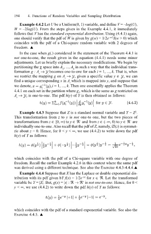
A → , is one-to-one. The pdf h(y) of Y is then obtained as follows:
i
Example 4.4.3 Suppose that Z is a standard normal variable and Y = Z .
2
This transformation from z to y is not one-to one, but the two pieces of
transformations from z ∈ [0, ∞) to y ∈ ℜ and from z ∈ (–∞, 0) to y ∈ ℜ are
+
+
individually one-to-one. Also recall that the pdf of Z, namely, ∅(z) is symmet-
ric about z = 0. Hence, for 0 < y < ∞, we use (4.4.2) to write down the pdf
h(y) of Y as follows:

which coincides with the pdf of a Chi-square variable with one degree of
freedom. Recall the earlier Example 4.2.6 in this context where the same pdf
was derived using a different technique. See also the Exercise 4.4.3-4.4.4.!
Example 4.4.4 Suppose that X has the Laplace or double exponential dis-
–|x|
tribution with its pdf given bY f(x) = 1/2e for x ∈ ℜ. Let the transformed
+
variable be Y = |X|. But, g(x) = |x| : ℜ → ℜ is not one-to-one. Hence, for 0 <
y < ∞, we use (4.4.2) to write down the pdf h(y) of Y as follows:

which coincides with the pdf of a standard exponential variable. See also the
Exercise 4.4.5. !