Page 231 - Probability and Statistical Inference

208 4. Functions of Random Variables and Sampling Distribution

Once the pdf h(w) is simplified in the case ν = 1, we find that h(w) = π –1
2 –1
(1+w ) for –∞ < w < ∞. In other words, when ν = 1, the Student’s t distri-
bution coincides with the Cauchy distribution. Verification of this is left as the
Exercise 4.5.2.

In some related problems we can go quite far without looking at
the pdf of the Student’s t variable. This point is emphasized next.

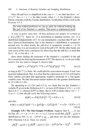
A case in point: note that –W thus defined can simply be written as
Since (i) –X is distributed as standard normal, (ii) –X is
distributed independently of Y, we can immediately conclude that W and –W
have identical distributions, that is the Student’s t distribution is symmetric
around zero. In other words, the pdf h(w) is symmetric around w = 0. To
conclude this, it is not essential to look at the pdf of W. On the other hand, one
may arrive at the same conclusion by observing that the pdf h(w) is such that
h(w) = h(–w) for all w > 0.
How about finding the moments of the Student’s t variable? Is the pdf
h(w) essential for deriving the moments of W? The answer is: we do not really
need it. For any positive integer k, observe that

as long as E[Y –k/2 ] is finite. We could split the expectation because X and Y are
assumed independent. But, it is clear that the expression in (4.5.2) will lead to
finite entities provided that appropriate negative moments of a Chi-square
variable exist. We had discussed similar matters for the gamma distributions
in (2.3.24)-(2.3.26).
By appealing to (2.3.26) and (4.5.2), we claim that for the Student’s t
variable W given in the Definition 4.5.1, we have E(W) finite if 1/2ν > –(–1/2)
2
that is if ν > 1, whereas E(W ) is finite, that is V(W) is finite when 1/2ν > –(–
1) or ν > 2. One should verify the following claims:

and also,

Example 4.5.1 The One-Sample Problem: Suppose that X , ..., X are
n
1
2
iid N(µ, σ ), –∞ < µ < ∞, 0 < σ < ∞, n ≥ 2. Let us recall that is
2
distributed as N(0, 1), (n – 1)S /σ is and these two are also indepen-
2
dent (Theorem 4.4.2). Then, we rewrite