Page 233 - Probability and Statistical Inference

210 4. Functions of Random Variables and Sampling Distribution

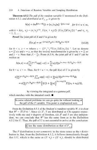
Theorem 4.5.2 The pdf of the random variable U mentioned in the Defi-
nition 4.5.2, and distributed as F í1, í2 , is given by

–1
with k = k(ν , ν ) = (ν /ν ) 1/2ν 1 Γ((ν + ν )/2) {Γ(ν /2)Γ(ν /2)} and ν , ν 2
1
2
1
2
2
1
1
1
2
= 1, 2, ... .
Proof The joint pdf of X and Y is given by
for 0 < x, y < ∞ where c = {2 (ν +ν )/2 Γ(ν /2)Γ(ν /2)} . Let us denote
–1
1
2
1
2
ν2
ν1
u = - x/y and v = y, so that the inverse transformation is given by x = - uv
ν2
ν1
ν1
and y = v. Note that |J| = - v. From (4.5.9), the joint pdf of U and V can be
ν2
written as
for 0 < u, v < ∞. Thus, for 0 < u < ∞, the pdf h(u) of U is given by

by viewing the integrand as a gamma pdf,
which matches with the intended result. ¢

In some related problems we can go quite far without looking at
the pdf of the F variable. This point is emphasized next.

From the Definition 4.5.1 of the Student’s t random variable W, it is clear
2
2
that W = X (Y/ν) . Since (i) X , Y are distributed as Chi-squares respec-
–1
2
2
tively with one and ν degrees of freedom, (ii) X and Y are also indepen-
2
dent, we can conclude that W has the same form as in the Definition
4.5.2 for U. Thus, the pdf of U is not essential to arrive at the conclusion:
has the same distribution as that of F
1, ν
The F distribution is not symmetric in the same sense as the t distri-
bution is. But, from the Definition 4.5.2, it follows immediately though
that 1/U, which is the same as (Y/ ν ) ÷ (X/ ν ), should be distributed
2 1