Page 242 - Probability and Statistical Inference

4. Functions of Random Variables and Sampling Distribution 219

The marginal distribution of each T has the Student’s t distribution with ν
i
degrees of freedom. This follows from the definition of the Student’s t ran-
dom variable. Jointly, however, (T , ..., T ) is said to have the p-dimensional
p
1
t distribution which depends on the correlation matrix ΣΣ ΣΣ Σ, denoted by Mt (ν,
p
Σ Σ Σ Σ Σ). One may refer to Johnson and Kotz (1972, p. 134). If we assume that
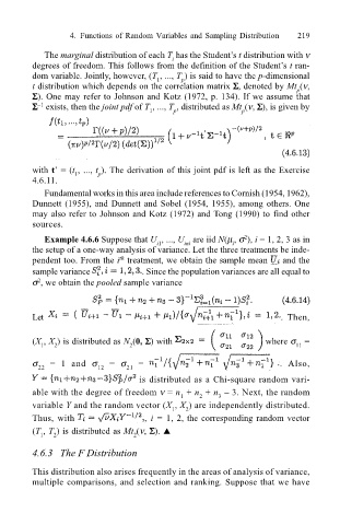
Σ Σ Σ Σ Σ exists, then the joint pdf of T , ..., T , distributed as Mt (ν, ΣΣ ΣΣ Σ), is given by
–1
p
1
p

with t’ = (t , ..., t ). The derivation of this joint pdf is left as the Exercise
1
p
4.6.11.
Fundamental works in this area include references to Cornish (1954, 1962),
Dunnett (1955), and Dunnett and Sobel (1954, 1955), among others. One
may also refer to Johnson and Kotz (1972) and Tong (1990) to find other
sources.

Example 4.6.6 Suppose that U , ..., U are iid N(µ , σ ), i = 1, 2, 3 as in
2
i1
i
ini
the setup of a one-way analysis of variance. Let the three treatments be inde-
pendent too. From the i treatment, we obtain the sample mean and the
th
sample variance . Since the population variances are all equal to
2
σ , we obtain the pooled sample variance
Let . Then,

(X , X ) is distributed as N (0, ΣΣ ΣΣ Σ) with where σ =
2
2
1
11
σ = 1 and σ = σ = . Also,
12
22
21
is distributed as a Chi-square random vari-
able with the degree of freedom ν = n + n + n – 3. Next, the random
1 2 3
variable Y and the random vector (X , X ) are independently distributed.
2
1
Thus, with , i = 1, 2, the corresponding random vector
(T , T ) is distributed as Mt (ν, ΣΣ ΣΣ Σ). !
1 2 2
4.6.3 The F Distribution
This distribution also arises frequently in the areas of analysis of variance,
multiple comparisons, and selection and ranking. Suppose that we have