Page 314 - Probability and Statistical Inference

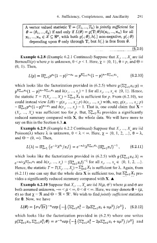
6. Sufficiency, Completeness, and Ancillarity 291

Example 6.2.8 (Example 6.2.1 Continued) Suppose that X , ..., X are iid
n
1
Bernoulli(p) where p is unknown, 0 < p < 1. Here, χ = {0, 1}, θ = p, and Θ =
(0, 1). Then,

which looks like the factorization provided in (6.2.5) where
and h(x , ..., x ) = 1 for all x , ..., x ∈ {0, 1}. Hence,
1 n 1 n
the statistic T = T(X , ..., X ) = is sufficient for p. From (6.2.10), we
1 n
could instead view L(θ) = g(x , ..., x ; p) h(x , ..., x ) with, say, g(x , ..., x ; p)
1
n
1
n
1
n
= and h(x , ..., x ) = 1. That is, one could claim that X =
1 n
(X , ..., X ) was sufficient too for p. But, provides a significantly
n
1
reduced summary compared with X, the whole data. We will have more to
say on this in the Section 6.3.!
Example 6.2.9 (Example 6.2.2 Continued) Suppose that X , ..., X are iid
n
1
Poisson(λ) where λ is unknown, 0 < λ < ∞. Here, χ = {0, 1, 2, ...}, θ = λ,
and Θ = (0, ∞). Then,
which looks like the factorization provided in (6.2.5) with
and h(x , ..., x ) = for all x , ..., x ∈ {0, 1, 2, ...}.
1 n 1 n
Hence, the statistic T = T(X , ..., X ) = is sufficient for λ. Again, from
1 n
(6.2.11) one can say that the whole data X is sufficient too, but pro-
vides a significantly reduced summary compared with X. !
Example 6.2.10 Suppose that X , ..., X are iid N(µ, σ ) where µ and σ are
2
1
n
both assumed unknown, –∞ < µ < ∞, 0 < σ < ∞. Here, we may denote θθ θθ θ = (µ,
σ) so that χ = ℜ and Θ = ℜ × ℜ . We wish to find jointly sufficient statistics
+
for θθ θθ θ. Now, we have
which looks like the factorization provided in (6.2.9) where one writes
and