Page 316 - Probability and Statistical Inference

6. Sufficiency, Completeness, and Ancillarity 293

To appreciate this fine line, let us think through the example again and
pretend for a moment that one could claim componentwise sufficiency. But,
since ( , S ) is jointly sufficient for (µ, σ ), we can certainly claim that
2
2
(S , ) is also jointly sufficient for θθ θθ θ = (µ, σ ). Now, how many readers
2
2
would be willing to push forward the idea that componentwise, S is suffi-
2
cient for µ or is sufficient for σ ! Let us denote U = and let g(u; n) be
2
the pdf of U when the sample size is n.

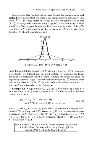
Figure 6.2.1. Two PDF’s of Where n = 16

In the Figure 6.2.1, the two pdf’s of when µ = 0 and n = 16, for example,
are certainly very different from one another. Relatively speaking, the darker
pdf gives the impression that σ is “small” whereas the lighter pdf gives the
impression that σ is “large”. There should be no doubt that provides some
information about σ . In fact has some information about both µ and σ ,
2
2
2
2
whereas S has information about σ alone. !
Example 6.2.13 Suppose that X , ..., X are iid Uniform(0, θ), where θ (>
n
1
0) is unknown. Here, χ = (0, θ) and Θ = ℜ . We wish to find a sufficient
+
statistic for θ. Now,
where x and x are respectively the observed smallest and largest order
n:1
n:n
statistics. The last step in (6.2.13) looks exactly like the Neyman factorization
provided in (6.2.5) where g(x ; θ) = θ I (0 < x < θ) and h(x , ..., x ) = I(0
–n
1
n
n:n
n:n
< x < x ) for all x , ..., x ∈ (0, θ). Hence, the statistic T = T(X , ..., X ) =
n:1 n:n 1 n 1 n
X is sufficient for θ. !
n:n
It is not crucial that the X’s be iid for the Neyman factorization
of the likelihood function to lead to a (jointly) sufficient
statistic (T)T. Look at the Example 6.2.14.