Page 333 - Probability and Statistical Inference

310 6. Sufficiency, Completeness, and Ancillarity

such statistics can play useful roles in statistical methodologies. In the mid
1920’s, R. A. Fisher introduced this concept and he frequently revisited it in
his writings. This concept evolved from Fisher (1925a) and later it blossomed
into the vast area of conditional inferences. In his 1956 book, Fisher empha-
sized many positive aspects of ancillarity in analyzing real data. Some of these
ideas will be explored in this and the next section. For fuller discussions of
conditional inference one may look at Basu (1964), Hinkley (1980a) and Ghosh
(1988). The interesting article of Reid (1995) also provides an assessment of
conditional inference procedures.
Consider the real valued observable random variables X , ..., X from some
1
n
population having the common pmf or pdf f(x; θ), where the unknown pa-
rameter vector θ belongs to the parameter space Θ ⊆ ℜ . Let us continue
p
writing X = (X , ..., X ) for the data, and denote a vector valued statistic by T
1
n
= T(X).
Definition 6.5.1 A statistic T is called ancillary for θ or simply ancillary
provided that the pmf or the pdf of T, denoted by g(t) for t ∈ , does not
involve the unknown parameter θ ∈ Θ.
Example 6.5.1 Suppose that X , ..., X are iid N(θ, 1) where θ is the
n
1
unknown parameter, –∞ < θ < ∞, n ≥ 3. A statistic T = X – X is distributed
2
1
1
as N(0, 2) whatever be the value of the unknown parameter θ. Hence T is
1
ancillary for θ. Another statistic T = X + ... + X – (n – 1)X is distributed
1
n–1
2
n
as N(0, n(n – 1)) whatever be the value of the unknown parameter θ. Hence
T is also ancillary for θ. The sample variance S is distributed as
2
2
whatever be the value of the unknown parameter θ and hence S is ancillary
2
too for θ. !
2
2
Example 6.5.2 Suppose that X , ..., X are iid N(µ, σ ), θ = (µ, σ ), –∞ <
1
n
µ < ∞, 0 < σ < ∞, n ≥ 2. Here both the parameters µ and σ are assumed
2
unknown. Let us reconsider the statistics T or T defined in the Example
1
2
2
6.5.1. Now, T , T are respectively distributed as N(0, 2σ ) and N(0, n(n –
1
2
2
1)σ ) respectively, and both these distributions clearly depend upon θ. Thus,
T or T is no longer ancillary for θ in this situation. The sample variance S is
2
1 2
distributed as and hence S is not ancillary either for θ. But,
2
2
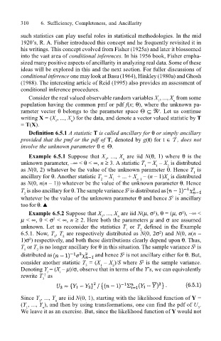
consider another statistic T = (X – X )/S where S is the sample variance.
1
3
2
Denoting Y = (X – µ)/σ, observe that in terms of the Y’s, we can equivalently
i
i
2
rewrite T as
3
Since Y , ..., Y are iid N(0, 1), starting with the likelihood function of Y =
n
1
(Y , ..., Y ), and then by using transformations, one can find the pdf of U .
n
1
3
We leave it as an exercise. But, since the likelihood function of Y would not