Page 334 - Probability and Statistical Inference

6. Sufficiency, Completeness, and Ancillarity 311

involve θ to begin with, the pdf of U would not involve θ. In other words, T 3
3
is an ancillary statistic here. Note that we do not need the explicit pdf of U to
3
conclude this. !
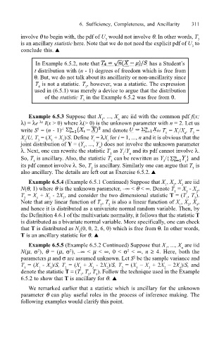
In Example 6.5.2, note that has a Student’s
t distribution with (n - 1) degrees of freedom which is free from
θ. But, we do not talk about its ancillarity or non-ancillarity since
T is not a statistic. T , however, was a statistic. The expression
3
4
used in (6.5.1) was merely a device to argue that the distribution
of the statistic T in the Example 6.5.2 was free from θ.
3
Example 6.5.3 Suppose that X , ..., X are iid with the common pdf f(x;
1
n
λ) = λe I(x > 0) where λ(> 0) is the unknown parameter with n = 2. Let us
–λx
write S = (n - 1) and denote T = X /X , T =
2
-1
1
n
2
1
X /U, T = (X + X )/S. Define Y = λX for i = 1, ..., n and it is obvious that the
1
3
3
2
i
i
joint distribution of Y = (Y , ..., Y ) does not involve the unknown parameter
1
n
λ. Next, one can rewrite the statistic T as Y /Y and its pdf cannot involve λ.
1 1 n
So, T is ancillary. Also, the statistic T can be rewritten as Y /{ Y } and
2
i
1
2
its pdf cannot involve λ. So, T is ancillary. Similarly one can argue that T is
3
2
also ancillary. The details are left out as Exercise 6.5.2. !
Example 6.5.4 (Example 6.5.1 Continued) Suppose that X , X , X are iid
2
1
3
N(θ, 1) where θ is the unknown parameter, –∞ < θ < ∞. Denote T = X - X ,
1
2
1
T = X + X - 2X , and consider the two dimensional statistic T = (T , T ).
1
2
2
2
3
1
Note that any linear function of T , T is also a linear function of X , X , X ,
1
2
1
2
3
and hence it is distributed as a univariate normal random variable. Then, by
the Definition 4.6.1 of the multivariate normality, it follows that the statistic T
is distributed as a bivariate normal variable. More specifically, one can check
that T is distributed as N (0, 0, 2, 6, 0) which is free from θ. In other words,
2
T is an ancillary statistic for θ. !
Example 6.5.5 (Example 6.5.2 Continued) Suppose that X , ..., X are iid
n
1
2
2
N(µ, σ ), θ = (µ, σ ), –∞ < µ < ∞, 0 < σ < ∞, n ≥ 4. Here, both the
2
parameters µ and σ are assumed unknown. Let S be the sample variance and
2
T = (X - X )/S, T = (X + X - 2X )/S, T = (X – X + 2X – 2X )/S, and
4
3
1
3
1
2
3
3
1
1
2
2
denote the statistic T = (T , T , T ). Follow the technique used in the Example
1
3
2
6.5.2 to show that T is ancillary for θ. !
We remarked earlier that a statistic which is ancillary for the unknown
parameter θ can play useful roles in the process of inference making. The
following examples would clarify this point.