Page 347 - Probability and Statistical Inference

6. Sufficiency, Completeness, and Ancillarity 324

Example 6.6.11 (Example 6.2.13 Continued) Suppose that X , ..., X are
n
1
iid Uniform(0, θ), θ(> 0) being the unknown parameter. We know that T(X) =
X is a minimal sufficient statistic for θ and the pdf of T is given by f(t; θ) =
n:n
nt θ I(0 < t < θ) which does not belong to the exponential family defined by
n-1 –n
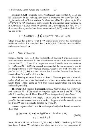
(6.6.9) with k = 1. But, we show directly that T is complete. Let h(t), 0 < t <
θ, be any arbitrary real valued function such that E [h(T)] = 0 for all θ > 0 and
θ
we can write

which proves that h(θ) ≡ 0 for all θ > 0. We have now shown that the minimal
sufficient statistic T is complete. See (1.6.16)-(1.6.17) for the rules on differ-
entiating an integral. !

6.6.2 Basu’s Theorem

Suppose that X = (X , ..., X ) has the likelihood function L which depends on
n
1
some unknown parameter ! and the observed value x. It is not essential to
assume that X , ..., X are iid in the present setup. Consider now two statistics
1
n
U = U(X) and W = W(X). In general, showing that the two statistics U and W
are independent is a fairly tedious process. Usually, one first finds the joint
pmf or pdf of (U, W) and then shows that it can be factored into the two
marginal pmf’s or pdf’s of U and W.
The following theorem, known as Basu’s Theorem, provides a scenario
under which we can prove independence of two appropriate statistics pain-
lessly. Basu (1955a) came up with this elegant result which we state here
under full generality.
Theorem 6.6.3 (Basu’s Theorem) Suppose that we have two vector val-
ued statistics, U = U(X) which is complete sufficient for θθ θθ θ and W = W(X)
which is ancillary for θθ θθ θ. Then, U and W are independently distributed.
Proof For simplicity, we supply a proof only in the discrete case. The
proof in the continuous situation is similar. Suppose that the domain spaces
for U and W are respectively denoted by U and W.
In order to prove that U and W are independently distributed, we need to
show that

Now, for w ∈ W, let us denote P (W = W) = h(W). Obviously h(W) is
θ
free from θ since W’s distribution does not involve the parameter θ.