Page 349 - Probability and Statistical Inference

6. Sufficiency, Completeness, and Ancillarity 326

any two sets A ⊆ ℜ, B ⊆ ℜ and we wish to verify that
+

We now work with a fixed but otherwise arbitrary value σ = σ (> 0). In this
0
situation, we may pretend that µ is really the only unknown parameter so that
we are thrown back to the setup considered in the Example 6.6.12, and hence
2
claim that is complete sufficient for µ and S is ancillary for µ. Thus,
having fixed σ = σ , using Basu’s Theorem we claim that and S will be
2
0
independently distributed. That is, for all µ ∈ ℜ and fixed σ (> 0), we have so
0
far shown that

But, then (6.6.12) holds for any fixed value σ ∈ ℜ . That is, we can claim
+
0
the validity of (6.6.12) for all (µ, σ ) ∈ ℜ × ℜ . There is no difference be-
+
0
tween what we have shown and what we started out to prove in (6.6.11).
Hence, (6.6.11) holds. !
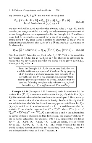
From the Example 6.6.15, the reader may think that we
used the sufficiency property of and ancillarity property
of S . But if µ, s are both unknown, then certainly is
2
not sufficient and S is not ancillary. So, one may think
2
that the previous proof must be wrong. But, note that we
used the following two facts only: when σ = σ is fixed
0
but arbitrary, is sufficient and S is ancillary.
2
Example 6.6.16 (Example 6.6.15 Continued) In the Example 6.6.15, the
statistic U = ( , S ) is complete sufficient for θ = (µ, σ ) while W = (X –
2
2
1
X )/S is a statistic whose distribution does not depend upon θ. Here, we may
2
use the characteristics of a location-scale family. To check directly that W
has a distribution which is free from θ, one may pursue as follows: Let Y =
i
(X – µ)/σ which are iid standard normal, i = 1, ..., n, and then note that the
i
statistic W can also be expressed as (Y - Y )/S* where S = (n – 1) -1
*2
1
2
with . The statistics U and W are independent
by virtue of Basu’s Theorem. In this deliberation, the ancillary statistic W
can be vector valued too. For example, with n ≥ 3, suppose that we define
W* = ({X – X }/S, {X – X }/|X + X – 2X |). As before, we can rewrite
1 2 2 3 1 2 3
W* as ({Y – Y }/S*, {Y – Y }/|Y + Y – 2Y |) where we recall that the Y’s
3
2
1
2
1
3
2
are iid standard normal, and hence W* is ancillary for θ. Hence, U and W*
are independent by virtue of Basu’s Theorem. !