Page 489 - Probability and Statistical Inference

466 9. Confidence Interval Estimation

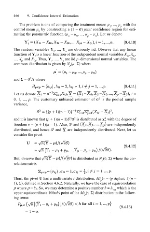
The problem is one of comparing the treatment means µ , ..., µ with the
p
1
control mean µ by constructing a (1 – σ) joint confidence region for esti-
0
mating the parametric function (µ – µ , ..., µ – µ ). Let us denote
1 0 p 0
The random variables Y , ..., Y are obviously iid. Observe that any linear
1
n
function of Y is a linear function of the independent normal variables X , X ,
i
2i
1i
..., X and X . Thus, Y , ..., Y are iid p–dimensional normal variables. The
pi
n
1
0i
common distribution is given by N (µ, Σ) where
p
2
and Σ = σ H where
Let us denote i =
2
0, 1, ..., p. The customary unbiased estimator of σ is the pooled sample
variance,

2
2
and it is known that (p + 1)(n – 1)S /σ is distributed as with the degree of
2
freedom v = (p + 1)(n – 1). Also, S and are independently
distributed, and hence S and are independently distributed. Next, let us
2
consider the pivot

But, observe that is distributed as N (0, Σ) where the cor-
p
relation matrix

Thus, the pivot U has a multivariate t distribution, Mt (v = (p + 1)(n –
p
1), Σ), defined in Section 4.6.2. Naturally, we have the case of equicorrelation
ρ where ρ = ½. So, we may determine a positive number h ≡ h which is the
v,α
upper equicoordinate 100α% point of the Mt (v, Σ) distribution in the follow-
p
ing sense: