
Page 571 - Probability and Statistical Inference
P. 571
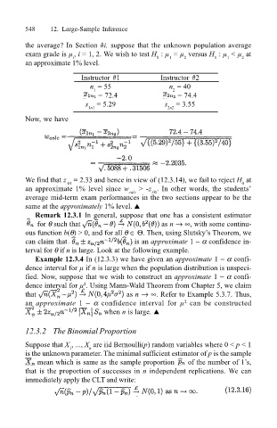
548 12. Large-Sample Inference
the average? In Section #i, suppose that the unknown population average
exam grade is µ , i = 1, 2. We wish to test H : µ = µ versus H : µ < µ at
1
1
2
2
i
0
1
an approximate 1% level.
Instructor #1 Instructor #2
n = 55 n = 40
1 2
= 72.4 = 74.4
s = 5.29 s = 3.55
1n1 2n2
Now, we have
We find that z = 2.33 and hence in view of (12.3.14), we fail to reject H at
.01
0
an approximate 1% level since w calc > -z . In other words, the students
.01
average mid-term exam performances in the two sections appear to be the
same at the approximately 1% level. !
Remark 12.3.1 In general, suppose that one has a consistent estimator
for θ such that as n → ∞, with some continu-
ous function b(θ) > 0, and for all θ ∈ Θ. Then, using Slutskys Theorem, we
can claim that is an approximate 1 − α confidence in-
terval for θ if n is large. Look at the following example.
Example 12.3.4 In (12.3.3) we have given an approximate 1 − α confi-
dence interval for µ if n is large when the population distribution is unspeci-
fied. Now, suppose that we wish to construct an approximate 1 − α confi-
dence interval for µ . Using Mann-Wald Theorem from Chapter 5, we claim
2
that as n → ∞. Refer to Example 5.3.7. Thus,
an approximate 1 − α confidence interval for µ can be constructed
2
when n is large. !
12.3.2 The Binomial Proportion
Suppose that X , ..., X are iid Bernoulli(p) random variables where 0 < p < 1
1
n
is the unknown parameter. The minimal sufficient estimator of p is the sample
mean which is same as the sample proportion of the number of 1s,
that is the proportion of successes in n independent replications. We can
immediately apply the CLT and write: