Page 566 - Probability and Statistical Inference

12. Large-Sample Inference 543

techniques are extended for analogous two-sample problems. These method-
ologies rely heavily upon the central limit theorem (CLT) introduced in Chap-
ter 5.

12.3.1 The Distribution-Free Population Mean

Suppose that X , ..., X are iid real valued random variables from a population
1
n
with the pmf or pdf f(x; θ) where the parameter vector θ is unknown or the
2
functional form of f is unknown. Let us assume that the variance σ = σ (θ)
2
of the population is finite and positive which in turn implies that the mean µ ≡
µ(θ) is also finite. Suppose that µ and σ are both unknown. Let
be respectively the sample
mean and variance for n ≥ 2. We can apply the CLT and write: As n → ∞,

From (12.3.1) what we conclude is this: For large sample size n, we should
be able to use the random variable as an approximate pivot
since its asymptotic distribution is N(0, 1) which is free from both µ, s.
Confidence Intervals for the Population Mean
Let us first pay attention to the one-sample problems. With preassigned α
∈ (0, 1), we claim that

which leads to the confidence interval

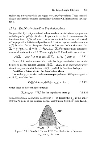
with approximate confidence coefficient 1 − α. Recall that z is the upper
α/2
100(α/2)% point of the standard normal distribution. See the Figure 12.3.1.

Figure 12.3.1. Standard Normal PDF: The Shaded Area Between
−z and z is 1 − α
α/2 α/2