Page 564 - Probability and Statistical Inference

12. Large-Sample Inference 541

Fisher (1922,1925a) gave the foundations of the likelihood theory. Cramér
(1946a, Chapter 33) pioneered the mathematical treatments under full gener-
ality with assumptions along the lines of A1-A3. One may note that the as-
sumptions A1-A3 give merely sufficient conditions for the stated large sample
properties of an MLE.
Many researchers have derived properties of MLE’s comparable to those
stated in (12.2.3)-(12.2.4) under less restrictive assumptions. The reader may
look at some of the early investigations due to Cramér (1946a,b), Neyman
(1949), Wald (1949a), LeCam (1953,1956), Kallianpur and Rao (1955) and
Bahadur (1958). This is by no means an exhaustive list. In order to gain
historical as well as technical perspectives, one may consult Cramér (1946a),
LeCam (1986a,b), LeCam and Yang (1990), and Sen and Singer (1993). Ad-
mittedly, any detailed analysis is way beyond the scope of this book.
We should add, however, that in general an MLE may not be consistent
for θ. Some examples of inconsistent MLE’s were constructed by Neyman
and Scott (1948) and Basu (1955b). But, under mild regularity conditions, the
result (12.2.3) shows that an MLE is indeed consistent for the parameter θ
it is supposed to estimate in the first place. This result, in conjunction with the
invariance property (Theorem 7.2.1), make the MLE’s very appealing in prac-
tice.
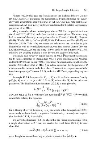
Example 12.2.1 Suppose that X , ..., X are iid with the common Cauchy
n
1
pdf f(x; θ) = π {1 + (x − θ) } I(x ∈ ℜ) where θ(∈ ℜ) is the unknown
2 -1
-1
parameter. The likelihood function from (12.2.1) is then given by

Now, the MLE of θ is a solution of the equation = 0 which
amounts to solving the equation

for θ. Having observed the data x , ..., x , one would solve the equation (12.2.5)
1
n
numerically with an iterative approach. Unfortunately, no analytical expres-
sion for the MLE is available.
We leave it as Exercise 12.2.1 to check that the Fisher information I (θ) in
a single observation is 2. Then, we invoke the result from (12.2.4) to con-
clude that

even though we do not have any explicit expression for !