Page 565 - Probability and Statistical Inference

542 12. Large-Sample Inference

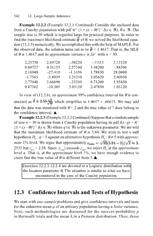
Example 12.2.2 (Example 12.2.1 Continued) Consider the enclosed data
from a Cauchy population with pdf π {1 + (x − θ) } I(x ∈ ℜ), θ ∈ ℜ. The
-1
2 -1
sample size is 30 which is regarded large for practical purposes. In order to
find the maximum likelihood estimate of θ, we solved the likelihood equa-
tion (12.2.5) numerically. We accomplished this with the help of MAPLE. For
the observed data, the solution turns out to be = 1.4617. That is, the MLE
of θ is 1.4617 and its approximate variance is 2n with n = 30.
-1
2.23730 2.69720 -.50220 -.11113 2.13320
0.04727 0.51153 2.57160 1.48200 -.88506
2.16940 -27.410 -1.1656 1.78830 28.0480
-1.7565 -3.8039 3.21210 5.03620 2.60930
2.77440 2.66690 -.23249 8.71200 1.95450
0.87362 -10.305 3.03110 2.47850 1.03120

In view of (12.2.6), an approximate 99% confidence interval for θ is con-
structed as which simplifies to 1.4617 ± .66615. We may add
that the data was simulated with θ = 2 and the true value of ? does belong to
the confidence interval. !
Example 12.2.3 (Example 12.2.2 Continued) Suppose that a random sample
of size n = 30 is drawn from a Cauchy population having its pdf f(x; q) = π -1
2 -1
{1 = (x - θ) } I(x ∈ ℜ) where q (∈ ℜ) is the unknown parameter. We are told
that the maximum likelihood estimate of θ is 5.84. We wish to test a null
hypothesis H : q = 5 against an alternative hypothesis H : θ ≠ 5 with approxi-
0 1
mate 1% level. We argue that approximately
2533 but z = 2.58. Since |z | exceeds z , we reject H at the approximate
calc
a/2
a/2
0
level a. That is, at the approximate level 1%, we have enough evidence to
claim that the true value of θ is different from 5.!
Exercises 12.2.3-12.2 4 are devoted to a Logistic distribution with
the location parameter θ. The situation is similar to what we have
encountered in the case of the Cauchy population.

12.3 Confidence Intervals and Tests of Hypothesis

We start with one-sample problems and give confidence intervals and tests
for the unknown mean µ of an arbitary population having a finite variance.
Next, such methodologies are discussed for the success probability p
in Bernoulli trials and the mean λ in a Poisson distribution. Then, these