Page 98 - Probability and Statistical Inference

2. Expectations of Functions of Random Variables 75

Example 2.2.4 Now, how should one evaluate, for example, E[(Z – 2) ]?
2
Use the Theorem 2.2.1 and proceed directly to write E[(Z – 2) ] = E[Z ] –
2
2
4E[Z] + 4 = 1 – 0 + 4 = 5. How should one evaluate, for example, E[(Z –
2)(2Z + 3)]? Again use the Theorem 2.2.1 and proceed directly to write E[(Z
2
– 2)(2Z + 3)] = 2E[Z ] – E[Z] –6 = 2 – 0 – 6 = –4. !
Next suppose that X has the N(µ, σ ) distribution with its pdf f(x) =
2
exp{–(x – µ) )/(2σ )} for –∞ < x < ∞, given by (1.7.13). Here we
2
2
recall that (µ, σ ) ∈ ℜ× ℜ .
2
+
Let us find the mean and variance of this distribution. One may be tempted
to use a result that (X – µ)/σ is standard normal and exploit the expressions
summarized in (2.2.25). But, the reader may note that we have not yet derived
fully the distribution of (X – µ)/σ. We came incredibly close to it in (1.7.18).
This matter is delegated to Chapter 4 for a fuller treatment through transforma-
tions and other techniques.
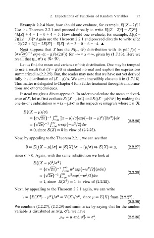
Instead we give a direct approach. In order to calculate the mean and vari-
2
2
ance of X, let us first evaluate E{(X – µ)/σ} and E{(X – µ) /σ } by making the
one-to-one substitution w = (x – µ)/σ in the respective integrals where x ∈ ℜ:

Now, by appealing to the Theorem 2.2.1, we can see that

since σ > 0. Again, with the same substitution we look at

Next, by appealing to the Theorem 2.2.1 again, we can write

We combine (2.2.27), (2.2.29) and summarize by saying that for the random
variable X distributed as N(µ, σ ), we have
2