Page 95 - Probability and Statistical Inference

72 2. Expectations of Functions of Random Variables

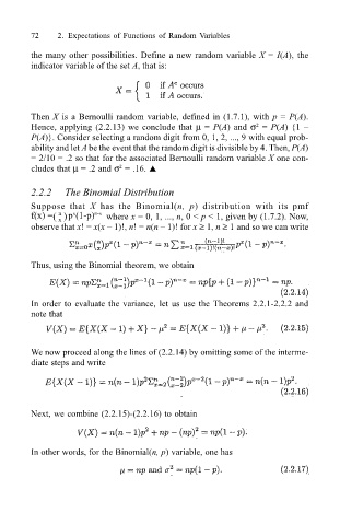
the many other possibilities. Define a new random variable X = I(A), the
indicator variable of the set A, that is:

Then X is a Bernoulli random variable, defined in (1.7.1), with p = P(A).
2
Hence, applying (2.2.13) we conclude that µ = P(A) and σ = P(A) {1 –
P(A)}. Consider selecting a random digit from 0, 1, 2, ..., 9 with equal prob-
ability and let A be the event that the random digit is divisible by 4. Then, P(A)
= 2/10 = .2 so that for the associated Bernoulli random variable X one con-
2
cludes that µ = .2 and σ = .16. !

2.2.2 The Binomial Distribution
Suppose that X has the Binomial(n, p) distribution with its pmf
n
f(x) = p (1-p) where x = 0, 1, ..., n, 0 < p < 1, given by (1.7.2). Now,
( )
x
n-x
x
observe that x! = x(x – 1)!, n! = n(n – 1)! for x ≥ 1, n ≥ 1 and so we can write
Thus, using the Binomial theorem, we obtain

In order to evaluate the variance, let us use the Theorems 2.2.1-2.2.2 and
note that

We now proceed along the lines of (2.2.14) by omitting some of the interme-
diate steps and write

Next, we combine (2.2.15)-(2.2.16) to obtain

In other words, for the Binomial(n, p) variable, one has