Page 90 - Probability and Statistical Inference

2. Expectations of Functions of Random Variables 67

where χ is the support of X. The expected value is also called the mean of the
distribution and is frequently assigned the symbol µ.
In the Definition 2.2.1, the term Σ i:xi ∈ χ x f(x ) is interpreted as the infinite
i
i
sum, x f(x ) + x f(x ) + x f(x ) + ... provided that x , x , x , ... belong to χ, the
1
2
3
2
3
1
support of the random variable X. 1 2 3
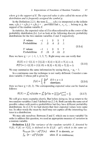
In statistics, the expected value of X is often referred to as the center of the
probability distribution f(x). Let us look at the following discrete probability
distributions for the two random variables X and Y respectively.

Here we have χ = y= {–1, 1, 3, 5, 7}. Right away one can verify that

We may summarize the same information by saying that µ = µ = 3.
X Y
In a continuous case the technique is not vastly different. Consider a ran-
dom variable X whose pdf is given by

Here we have χ = (0, 2). The corresponding expected value can be found as
follows:

We will give more examples shortly. But before doing so, let us return to the
two random variables X and Y defined via (2.2.4). Both can take the same set of
possible values with positive probabilities but they have different probability
distributions. In (2.2.5) we had shown that their expected values were same
too. In other words the mean by itself may not capture all the interesting fea-
tures in a distribution.
We may ask ourselves: Between X and Y, which one is more variable? In
order to address this question, we need an appropriate measure of variation in
a random variable.
Definition 2.2.2 The variance of the random variable X, denoted by
2
V(X), V{X} or V[X], is defined to be E{(X – µ) } which is the same as: