Page 89 - Probability and Statistical Inference
P. 89
66 2. Expectations of Functions of Random Variables
be {8n 2(k n )}/k which is rewritten as follows:
k k
What will W amount to when k is very large? Interpreting probabilities as the
k
limiting relative frequencies we can say that should coincide with the
probability of seeing the face six in a single roll of a fair die which is nothing
but 1/6. Hence, the players ultimate win per game is going to be
In other words, in this game the player will lose one-third of a dollar in the long
run. It is seen readily from (2.2.2) that we multiplied the possible value of the
win with its probability and added up these terms.
In (2.2.2), the final answer is really the weighted average of the two pos-
sible values of the win where the weights are the respective probabilities. This
is exactly how we interpret this players expected win (per game) in the long
haul. The process is intrinsically a limiting one and in general we will proceed
to define the expected value of a random variable X as simply the weighted
average of all possible values of the random variable. More precise statements
would follow.
Let us begin with a random variable X whose pmf or pdf is f(x) for x ∈ ⊆ χ
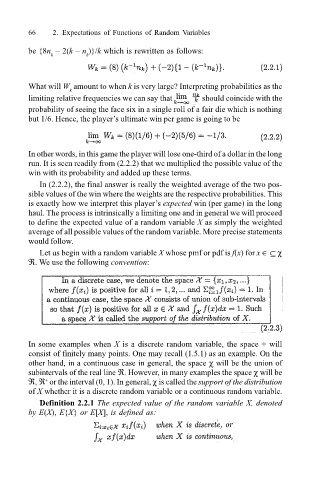
ℜ. We use the following convention:
In some examples when X is a discrete random variable, the space ÷ will
consist of finitely many points. One may recall (1.5.1) as an example. On the
other hand, in a continuous case in general, the space χ will be the union of
subintervals of the real line ℜ. However, in many examples the space χ will be
ℜ, ℜ or the interval (0, 1). In general, χ is called the support of the distribution
+
of X whether it is a discrete random variable or a continuous random variable.
Definition 2.2.1 The expected value of the random variable X, denoted
by E(X), E{X} or E[X], is defined as:

