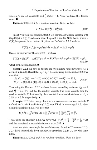
Page 92 - Probability and Statistical Inference

2. Expectations of Functions of Random Variables 69

since a ‘s are all constants and ∫ f(x)dx = 1. Now, we have the desired
χ
i
result.!
Theorem 2.2.2 Let X be a random variable. Then, we have

Proof We prove this assuming that X is a continuous random variable with
its pdf f(x), x ∈ χ. In a discrete case, the proof is similar. Note that µ, which is
E(X), happens to be a constant. So, from the Definition 2.2.2 we have

Hence, in view of the Theorem 2.2.1, we have

which is the desired result. !
Example 2.2.1 We now go back to the two discrete random variables X, Y
defined in (2.2.4). Recall that µ = µ = 3. Now, using the Definition 2.2.3 we
Y
X
note that

Then using the Theorem 2.2.2, we have the corresponding variances 4.8
and = 7.6. We find that the random variable Y is more variable than the
random variable X. Incidentally, the associated standard deviations are σ ≈
X
2.19, σ ≈ 2.76 respectively. !
Y
Example 2.2.2 Next we go back to the continuous random variable X
defined in (2.2.6). Recall from (2.2.7) that X had its mean equal 1.5. Next,
using the Definition 2.2.3 we note that

Thus, using the Theorem 2.2.2, we have
and the associated standard deviation is σ ≈ .387. !
X
Next, we state two simple but useful results. Proofs of Theorems 2.2.3-
2.2.4 have respectively been included as Exercises 2.2.18-2.2.19 with some
hints.
Theorem 2.2.3 Let X and Y be random variables. Then, we have