Page 366 - Process Modelling and Simulation With Finite Element Methods

A MATLAB/FEMLAB Primer for Vector Calculus 353

where 0 is the angle between the vectors a and b. To achieve the same result in
MATLAB, we use the * operator
>> a = [l; 2; 31;
>> b = [-3 2 -11;
>> b*a
ans =
-2

This is a special case of a row vector (1 x 3 matrix) multiplying a column vector
(3 x 1 matrix). As the first dimension of the latter and the second dimension of
the former are the same, these matrices are compatible and can be multiplied
according to the general rule for matrix multiplication

j=1
If A is an mx II matrix and B is an IZX 1 matrix, then AB is an mx 1 matrix. If the
common size is not respected, then the matrices are incompatible and the product
is not defined. MATLAB can compute scalar products as the special case of
matrix multiplication, but care must be taken to respect compatibility of the
vectors. For instance,
>> a*b
ans =
-3 2 -1
-6 4 -2
-9 6 -3
What happened? Simply, a is a 3 x 1 matrix multiplying a 1 x 3 matrix, b. The
product, ab, is a 3 x 3 matrix, viz.

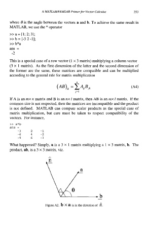
Figure A2. b X a is in the direction of 6.