Page 365 - Process Modelling and Simulation With Finite Element Methods

352 Process Modelling and Simulation with Finite Element Methods

a = a,i + a2j + a3k
(A1)
a = (apu2,a3)

where i, j and k are unit vector in the coordinate directions, a, , a2 , a3 are the
components of a relative to this set of axes. They are the projections of a on
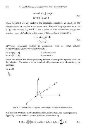
to the unit vectors i, jandk . For a point P with coordinates (x,y,z), the
position vector of P relative to the origin of the coordinate system, 0, is
r = xi + yj + zk
(A2)
= (X’ Y ’ z)

MATLAB represents vectors in component form as either column
(countervariant) or row (covariant) vectors:
>> a = [l; 2; 31; % column vector
>>a= [l 2 31; 70 row vector
In the row vector, the white space (any number of contiguous spaces) serves as
the delimiter. The column vector is delimited by semicolons, or alternatively, by
newlines:
>>a=[l
2
31;

fZ

dx
Figure Al. Position vector of a point P with respect to Cartesian coordinate axes.

A. 1.2 Scalar products, matrix multiplication, unit vectors, and vector products
Typically, scalar products (or dot products) are defined by
3
a.b=la1161cos6=a,b,+a2b,+a3b, =zaibi (‘43)
i=l