Page 360 - Process Modelling and Simulation With Finite Element Methods

Electrokinetic Flow 347

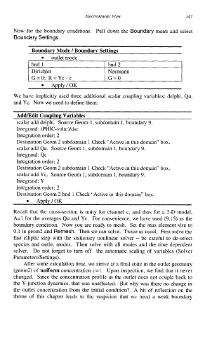
Now for the boundary conditions. Pull down the Boundary menu and select
Boundary Settings.

bnd 1 bnd 2
Dirichlet Neumann
G=0; R=Yc-c G=O

We have implicitly used three additional scalar coupling variables: delphi, Qu
and Yc. Now we need to define them:

Adadit Coupling Variables
scalar add delphi. Source Geom 1, subdomain 1, boundary 9.
Integrand: (PHIC-voltc)/dsc
Integration order: 2
Destination Geom 2 subdomain 1 Check “Active in this domain” box.
scalar add Qu. Source Geom 1, subdomain 1, boundary 9.
Integrand: Qc
Integration order: 2
Destination Geom 2 subdomain 1 Check “Active in this domain” box.
scalar add Yc. Source Geom 1, subdomain 1, boundary 9.
Integrand: Y
Integration order: 2
Destination Geom 2 bnd 1 Check “Active in this domain” box.

Recall that the cross-section is unity for channel c, and thus for a 2-D model,
A=l for the averages Qu and Yc. For convenience, we have used (9.15) as the
boundary condition. Now you are ready to mesh. Set the max element size to
0.1 in geom2 and Remesh. Then we can solve. Twice as usual. First solve the
fast elliptic step with the stationary nonlinear solver - be careful to de-select
species and outlet modes. Then solve with all modes and the time dependent
solver. Do not forget to turn off the automatic scaling of variables (Solver
ParameterdSettings).
After some calculation time, we arrive at a final state in the outlet geometry
(geom2) of uniform concentration c=l. Upon inspection, we find that it never
changed. Since the concentration profile in the outlet does not couple back to
the Y-junction dynamics, that was unaffected. But why was there no change in
the outlet concentration from the initial condition? A bit of reflection on the
theme of this chapter leads to the suspicion that we need a weak boundary