Page 359 - Process Modelling and Simulation With Finite Element Methods

346 Process Modelling and Simulation with Finite Element Methods

First of all, now that the downstream spatial variation of species is available
from the segment c solution, an improved boundary condition for the junction
domain at the outflow boundary is possible. One can impose the computed
segment species gradient over the entire outflow boundary:

(9.16)

This corresponds to a uniform average diffusion flux over the outflow boundary
for the junction computation and ensures balance of diffusion mass flow rate of
the species at c. It remains to enforce mass balance for the other two species
mass flux processes, convection and electrophoresis. Doing so leads to the
boundary condition for Eq. 9.14:

a@ @c -@c
=
Here, it should be noted that - . If this is not strictly correct, as
as hs,
will be the case for non-uniform electrical conductivity, one must solve the one-
dimensional equation for potential along with 9.14.

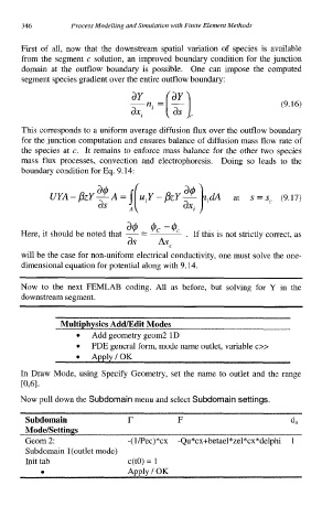
Now to the next FEMLAB coding. All as before, but solving for Y in the
downstream segment.

Multiphysics Add/Edit Modes
0 Add geometry geom2 1D
PDE general form, mode name outlet, variable c>>
0
0 Apply/OK
In Draw Mode, using Specify Geometry, set the name to outlet and the range
[0,61.
Now pull down the Subdomain menu and select Subdomain settings.

Subdomain r F da
Mode/Settings
Geom 2: -( l/Pec)*cx -Qu*cx+betael*zel*cx*delphi 1
Subdomain 1 (outlet mode)
Init tab c(t0) = 1
Apply / OK
0