Page 358 - Process Modelling and Simulation With Finite Element Methods

Electrokinetic Flow 345

elliptic step and time dependent restarts. The loop is then placed around the
second set of solutions. The final part is to append the fem.so1 structure with the
current set of solution vectors and tlist. Now run the animation to appreciate the
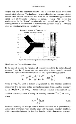
speed and electrokinetic switching in action. Figure 9.11 shows the
configuration in the “lower” pseudosteady state (second half period). The
striking feature of the animation is how reproducible each cycle is - diffusion
does not smooth anything out cumulatively.
Time=12 Color: Y Contour: phi
Arrow: velocitv vector Max 13 MBX 101

-2 1 a 1 2 3 4 MI” r 52~m -5~8~.0c
Figurr: 9 11 Lower flow pattern in the second half-period
Monitoring the Outpiit Concentration

In the case of species, the variation of concentration along the outlet channel
segment C may be of interest and one must solve at least a one-dimensional
differential equation for species distribution. The equation for this case is:

(9.14)

where b’ = Q,/A and s is distance along channel C. The boundary condition
at reservoir C is the same as that used at the junction domain outflow boundary
c, i.e. dY/& = 0 at s = sC. At the upstream boundary of the segment one

could take the simple route of setting the boundary condition Y = Y, at s = S,
where
Y, =-jYdA
1
(9.15)
A,
However, imposing this average value of mass fraction will not in general satisfy
conservation of species. Carc must be taken with the species boundary condition
at thc connection between the junction domain and the downstream segment.