Page 354 - Process Modelling and Simulation With Finite Element Methods

Electrokinetic Flow 341

is found, an improvement over the logical function method, but at an inordinate
price.
By the way, you might have found our choice of how to code the coupling
variables in terms of either the logical functions or square wave as long-winded.
The reason for not using the coding with greatest algebraic simplicity was to
insure that our initial step of the fast elliptic solution finds the correct initial
conditions. By trial and error, we learned that any MATLAB function with t as
an independent variable evaluates to zero when using the stationary nonlinear
solver. It does not substitute t=O into the formula, but rather chucks out the
function altogether. By coding as we did, the correct t=O conditions are found
(either PHIA or PHIB) in spite of this quirk.

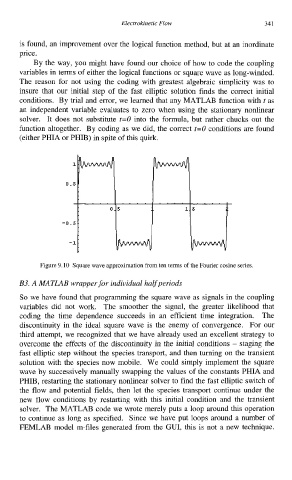
Figure 9.10 Square wave approximation from ten terms of the Fourier cosine series.
B3. A MATLAB wrapper for individual halfperiods

So we have found that programming the square wave as signals in the coupling
variables did not work. The smoother the signal, the greater likelihood that
coding the time dependence succeeds in an efficient time integration. The
discontinuity in the ideal square wave is the enemy of convergence. For our
third attempt, we recognized that we have already used an excellent strategy to
overcome the effects of the discontinuity in the initial conditions - staging the
fast elliptic step without the species transport, and then turning on the transient
solution with the species now mobile. We could simply implement the square
wave by successively manually swapping the values of the constants PHIA and
PHIB, restarting the stationary nonlinear solver to find the fast elliptic switch of
the flow and potential fields, then let the species transport continue under the
new flow conditions by restarting with this initial condition and the transient
solver. The MATLAB code we wrote merely puts a loop around this operation
to continue as long as specified. Since we have put loops around a number of
FEMLAB model m-files generated from the GUI, this is not a new technique.