Page 350 - Process Modelling and Simulation With Finite Element Methods

Electrokinetic Flow 331

they are inhomogeneous as here. The inhomogeneous Dirichlet conditions for u
and v, however, are constraints and so require the weak boundary treatment to
bring out the full nonlinearity and coupling.
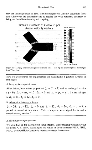
Time=l Sutface: Y Contour: phi
Arrow: velocity vectors Max 5 Max 101
1
09
15
08
1
07
05 06
0 05
04
-0 5
03
1
02
-1 5 01
-2 0
-1 0 1 2 3 4 Min 0 Min -000186
Figure 9 8 Merging concentration profile after unit time -- each leg has a forming front that merges
in th Y-junction

Now we are prepared for implementing the microfluidic Y-junction switcher in
two stages:
A. Merging two input streams

All as before, but uniform properties (c,. = Or = 1) with an uncharged species
(z=O). Asa =Asb =lo, Asc =6 and pA =pB =pc. Set the voltages
to $A =24, $B -12, $c =O.

B. Alternation between voltages
=24, GB -12, $,=O and $A =12, GB = 24, $c =o with a
period of around 6 time units. This is a square wave signal for A and a
complementary one for B .

A. Merging two input streams
We are all set up for merging two input streams. The constant potentials are set
for nodes A, B, and C according to the values of three constants PHIA, PHIB,
PHIC. Use Add/Edit Constants to introduce these three values.